Cross-account AWS FSx for Lustre and S3 data repository associations

FSx for Lustre and S3 are two complementary methods of storing data in Amazon Web Services (AWS). FSx offers an extremely performant, reliable, true filesystem, but it’s expensive and not accessible via the web or other APIs. S3 offers cheaper object storage that’s accessible from any device connected to the internet, but methods to access objects in S3 as files are limited.

AWS does have a great feature where you can set up a data repository association between a FSx for Lustre filesystem and n S3 bucket. This lets you sync the contents of the filesystem and the bucket, either in one direction or bidirectionally. This is helpful for users who want to access data from a traditional file path on a filesystem, but the data lives in S3. It’s also good if users also want to output results onto the filesystem, but other teams want to access the results from S3.

AWS supports linking FSx and S3 resources in different accounts, and even in different regions (FSx to S3 export only). However, nowhere in the documentation does AWS cover how to configure permissions to enable cross-account data repository associations.

At Deep Origin, we just set this up to let one of our customers access data in a S3 bucket as files in a ComputeBench. I wanted to share a simplified version of bucket polices in case anyone was searching the internet for the same answer!

To access a bucket via the “import” read-only data repository association, add this policy to the source bucket. Change YOUR_BUCKET to the id of the source bucket, and ACCOUNT_WITH_FSx:user/USER to the IAM identifier of the account owning the FSx volume. You can then set up the data repository association from the account owning the FSx volume as you normally would.

{
    "Version": "2012-10-17",
    "Statement": [
        {
            "Effect": "Allow",
            "Action": [
                "s3:Get*",
                "s3:List*",
                "s3:PutBucketNotification"
            ],
            "Resource": [
                "arn:aws:s3:::YOUR_BUCKET/*",
                "arn:aws:s3:::YOUR_BUCKET"
            ],
            "Principal": {
                "AWS": "arn:aws:iam::ACCOUNT_WITH_FSx:user/USER"
            }
        }
    ]
}


For a bucket policy that also allows export of data from FSx to S3, add a few write permissions:


{
    "Version": "2012-10-17",
    "Statement": [
        {
            "Effect": "Allow",
            "Action": [
                "s3:Get*",
                "s3:List*",
                "s3:PutBucketNotification",
                "s3:AbortMultipartUpload",
                "s3:DeleteObject",
                "s3:PutObject",
            ],
            "Resource": [
                "arn:aws:s3:::YOUR_BUCKET/*",
                "arn:aws:s3:::YOUR_BUCKET"
            ],
            "Principal": {
                "AWS": "arn:aws:iam::ACCOUNT_WITH_FSx:user/USER"
            }
        }
    ]
}

Getting a industry job after grad school

You’ve decided to move on from the academic career path after finishing your masters or PhD. Congratulations! However, making the transition out of academia can be hard, intimidating, and lonely. There are so many possible paths, rather than the linear grad school to postdoc to faculty pipeline, and it can feel like you’re leaving your community behind after years in the university system. Here’s some advice that helped me with the transition to my first biotechnology job, and a few things I learned hiring scientists and managing a team at Loyal and Formic Labs. This advice is based on my own experience and the experiences of the people close to me – it won’t be perfectly applicable to fields outside of biotechnology. I’ll cover three key areas: how to find the right position, how to apply and get the job, and how to find your people.

How to find the right position

Narrow down your search space as much as possible

There are over three thousand biotech companies in the Bay Area alone. That’s a huge number compared to the 5-10 schools offering graduate biology degrees. Your first task is to narrow the search space using a few key factors.

  1. What field do you want to work in? Maybe your PhD research was in gene therapy delivery, and you’d like to stay in that space. Congrats, you just narrowed your search space down to only 88 companies in CA (data from BioPharmGuy, considering gene therapy, RNA and peptide therapy companies).
  2. What company size would you enjoy most? This can be a hard question to answer if you haven’t had a non-academic job before, but you can use clues from grad school. Knowing what you know now, what type of lab would you ideally want to work in? One with a small team and hands-on advisor, or a large lab with many graduate students and postdocs, but limited attention from your advisor? Are you excited or frightened by the idea of working in a new lab with a young advisor, before they’ve gotten tenure? The answers to these questions can steer you towards small and big companies, and towards or away from startups.
  3. Where do you want to live? Geography is an important consideration that shouldn’t be ignored. You now have the flexibility of being independent of the university system – use it to make a choice based on cost of living, proximity to family and friends, hobbies, or the best place to raise a family. Depending on the industry, your best options may be in one of a few hubs.
  4. Do you want to work remotely? If you enjoy the tradeoffs of remote work, limit your search to positions that offer this up front. Companies will often bring the entire team together a few times a year, so be prepared to travel at least at least a few times if you go down this route.

Talk to as many people as you can

You can start this process while you’re still in grad school. It’s not uncommon or uncool to do “informational interviews” with people in your field. These people might be a lab or university alumni, someone who has published in the same research area, or even just someone you follow online. I’ve had great luck in reaching out to strangers on Twitter or Linkedin to talk about ideas and careers.

Search smarter, not harder

Two websites I’ve already linked hold databases of biotech companies and a biotech-specific job board: BioPharmGuy and BioSpace. Searching on these sites can be great for both company discovery and job postings. AngelList Talent can help with the search for jobs at newer startups.

Get on Twitter

Twitter is a hub for science information, new publications, job postings, and gossip in the field. Especially for the startup scene, Twitter has far more value than Linkedin. You don’t even have to post anything, just find some interesting people to follow and go from there. The #AltAcChats hashtag is a good place to start.

Your skills are general – it’s okay to change fields

The skills you learn during a PhD are more generally applicable than you may believe. Did you manage projects involving several lab members or outside collaborators? Did you mentor undergrads or new members of the lab? TA and develop material for a course? Take on a project in a new research area after jumping into the deep end of the literature pool? Recognize, promote, and sell these skills – they are valuable in any field you end up committed to. Conquering a PhD means you can learn pretty much anything.

Get connected with the venture capitalists

The best VCs have an expert birds-eye-view of their industry, and they have an incentive to place talented people at their portfolio companies. I’ve talked with VCs from Lux Capital, 8VC, Northpond and others at biotech meetups. They’re always looking to network with talented people – they need dealflow just as much as you need a job or a term sheet!

Consider roles outside of pure research

Consider strategic operations, chief of staff, project management, VC, and other “alternative” roles. If you love being involved with science but don’t see yourself doing pure research forever, there are many ways to stay involved without opening a lab notebook.

How to apply and get the job

Your resume, cover letter, or intro needs to stand out

If you’ve identified a company and role that is a good fit for you, and you want to apply, realize that hiring managers get A LOT of resumes. This is especially true when a job is posted on Linkedin or other general job sites. If a manager only has a minute or two to devote to each resume, you have to stand out in a positive way. Maybe it’s a relevant and interesting thesis title, an open source software project you’ve contributed to, or a good word from someone working at the company. Any positive connection or good word can go a long way to getting you a first interview.

Do many, many interviews

Especially if you’re unfamiliar with the interview process, or they make you nervous. It might seriously suck at first, but the only way to get more comfortable with interviewing is to put yourself out there and get uncomfortable. In the age of zoom, you can interview with a company halfway across the country without ever leaving your room (or putting on pants). I’ll even suggest doing earlier interviews with companies that you may be a good fit for, but you know you wouldn’t take. You’ll learn some of the common interview questions, get practice summarizing your research experience, and learn about the salary bands for the role (you are going to ask about salary, right?)

Have something to show in public, especially if you’re interviewing for a computational or software role

This could be a personal website, Github repository, a website for a side project, or a reproducible demo analysis from a paper. You want something that can show off your programming and quantitative skills from any device connected to the internet. Be prepared to walk through design choices for the code and any areas that were particularly interesting or challenging. Good documentation is important for any software intended to be re-used – docs are valued more in industry than in academia.

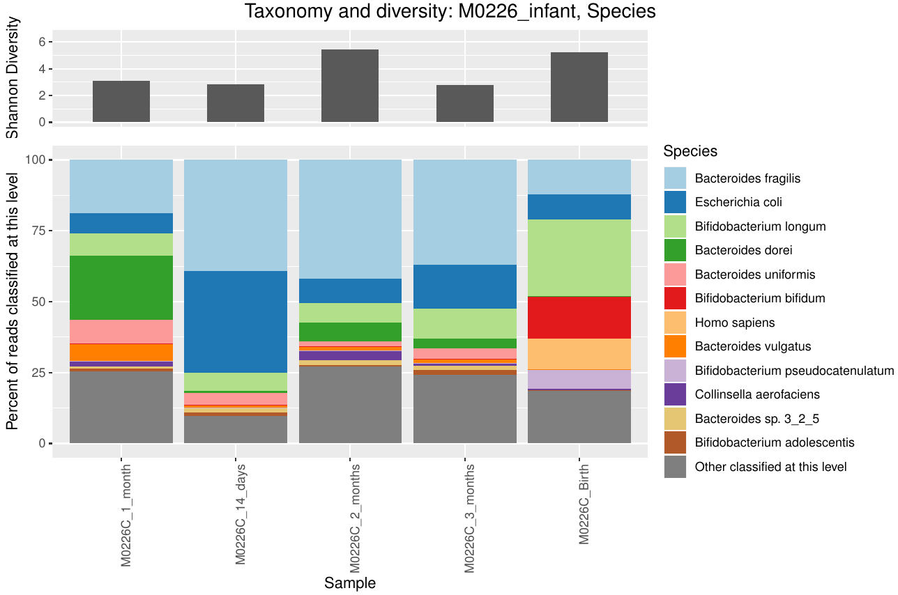
I have a few personal examples that I’ve repeatedly sent in messages or brought up live on a zoom interview. The bhattlab_workflows and kraken2_classification pipelines are not miracles of software engineering by any means, but they’re still used by members of the Bhatt lab and others, they make nice figures, and they have good docs. My bioinformatics in the cloud post is now a few years out of date, but it shows that I have been thinking about the challenges and solutions in this field for a while.

Brush up on the latest trends, languages, and frameworks in your field

In bioinformatics, Nextflow is the most popular workflow manager, and cloud compute skills are a necessity. Being familiar with both of these tools will help any bioinformatics interview. So, re-write a simple pipeline from grad school in Nextflow, sign up for the AWS Free Tier, and learn how to deploy it to AWS Batch. You could even write a blog post or a Twitter thread about the process, what you learned, and what you found challenging, then refer to it during an interview. A weekend of work will set you apart from those who haven’t tried to make the transition.

Utilize resources at your university

Many universities have free career counseling or job boards for people in situations just like you! Make sure you take advantage of these resources. You could probably benefit from a resume review, Linkedin profile checkup, or just someone knowledgeable to talk through your different options with.

Know what you’re worth. Negotiate.

Salary and equity compensation is field and role dependent. Talking with others in positions you’re applying to is the best way to get the current numbers. Ask for a range rather than direct numbers to avoid getting too personal. Also, recognize the tradeoffs that come with company size. Startups can’t pay as well, but can compensate with equity that could be life-changing in the event of a successful exit. Later-stage or public companies will be more stable and offer more in salary without the asymmetric upside. Finally, realize an offer is just a starting point for negotiations. There’s a hard limit for every position, but most offers can be flexed for the right candidate. You can also trade salary for equity (and vice-versa) depending on your risk tolerance.

How to find your people

Find your in-person community

There are growing meetup groups for young scientists in biotech and other fields. Right now, I’m seeing these mostly advertised in the Bay Area, NYC, and Boston, but they’re rapidly expanding to other areas as well. My top two for the Bay are Bits in Bio (which also has an active Slack community with over 2000 members) and Ergo Bio’s Biotech Venture Meetups. Groups like Nucleate bring together biotech founders from around the world.

Find your online community

I feel like the network of people talking about industry jobs, trends, and advice is stronger than ever. Twitter and Slack spaces like Bits in Bio are full of friendly and talented people.

Don’t stress about finding the “perfect” industry position in your first role out of grad school

Industry is not like academia, where you must commit 4+ years to a single field, and where your life is defined by your research area. You will learn more than you expect in the first year of your new role, and if you’re not happy, you’ll be in a better place to change it a year in. It’s much easier to change jobs in industry, and each change can come with better fit and increased compensation.

Rare transmission of commensal and pathogenic bacteria in the gut microbiome of hospitalized adults (2)

When we last left off, I was peering into the -80 freezer at the hundreds of stool samples I would need to analyze. In reality, a lot of experimental design work came on this project before I ever opened up the freezer!

Designing a good experiment was one of the most important things I learned in grad school. Science is already hard enough – you need to set yourself up for success from the beginning by designing a good experiment, whether it’s wet lab or computational. I like to think about what success in this project would look like, and work backwards from success to understand the data I need to collect.

To convincingly prove that a bacterium had transmitted from the microbiome of one patient to the microbiome of another, I needed the following pieces of evidence:

  1. At a given point in time, the bacterial genome was present in the microbiome of the source patient and undetectable in the microbiome of the recipient.
  2. At a future point in time, the bacterial genome was present in the microbiome of the recipient patient, and ideally persisted for multiple future time points.

Through Stanford Hospital, I also had access to a dataset of each patient’s room history. From this, I could find when two patients were roommates. Mapping the overlapping intervals, combined with the list of samples biobanked from each patient, was a challenging data science problem. It took me about a month of work to design an experiment that would give me the best chance of observing patient-patient microbiome transmission, if it was happening.

The wet lab work for this project was long and monotonous. You can read about it in the methods section of the paper, but we did DNA extraction and 10X Genomics linked read sequencing on all of the new samples.

When the new data came back, it was time to get cracking! The processing pipeline and data analysis I had planned would take too long to run on Stanford’s HPC cluster, so I turned to Google Cloud to get everything done with quick parallelization. The process of getting our workflows to run at scale in the cloud was certainly a learning experience, and I wrote a blog post about the effort (two years ago).

After assembling bacterial genomes from hundreds of microbiome samples, comparing strain-level populations with inStrain, and generating massive matrices comparing all sets of genomes in my samples, the true data analysis began. A few key lessons from the data analysis and writing experience have stuck with me, and the challenges made me a better scientist.

  1. Scrutinize your results! When I initially looked for identical bacterial genomes in samples from different patients, I found many “transmission events” that were simply the results of barcode swapping (when samples sequenced on an Illumina machine at the same time experience a small degree of contamination). I was prepared for this outcome, and developed a method to quantify when identical genomes were likely the result of barcode swapping in the linked read data.
  2. Carefully evaluate negative findings. After eliminating all the likely false positive results, I found very few identical genomes between patients, especially antibiotic resistant pathogens. At first, this was an upsetting result. I was really hoping to find lots of transmission between patients who were roommates! However, the lack of pathogen transmission findings allowed me to focus on the potentially more interesting cases of commensal bacteria transmitted between patients. The “negative” finding here turned out to make a more interesting story.


Tail risk hedging – replication of the VXTH index

In my last post about hedging a portfolio with options, I looked at how a complicated 4-option spread could replicate the VIX index and hedge against market volatility. Now, we’re going to look at a simpler, explicit “tail risk” hedge using VIX calls. This strategy is based on the VXTH index (VIX Tail Hedge), which buys 30 delta VIX calls with 1% of the portfolio when volatility is low, and allocates the rest into the SPX index. Looking at the performance of the index below, three things are immediately clear:

  1. VXTH did well, but not stellar, in 2008-2009
  2. VXTH slightly underperformed the benchmark during the bull market of 2010-2020
  3. VXTH absolutely skyrocketed during the COVID crash of 2020. I think this played right into the strengths of the hedging program: a rapid VIX spike, followed by quick recovery of SPX.

We’re going to look at replicating the VXTH index and extending the methodology to other portfolios, including a leveraged ETF portfolio holding UPRO and TMF.


Equity curves of VXTH (green) compared to SPX (black) from 2006-2020.

How does VXTH work?

The methodology is simple. Each month, the look at the front month VIX futures contract and decide how to allocate to the hedge. With the specified fraction of the portfolio, buy 30 delta VIX calls with one month to expiration.

VIX future valuePortfolio allocation
X <= 150%
15 > X <= 30 1%
30 > X <= 500.5%
X > 500%

N.B. The phrase “forward value of VIX” on the CBOE website is strange and doesn’t have an explicit meaning (at least to me). I confirmed the index is looking at the front month VIX future rather than spot VIX by examining the trade log on the CBOE website.

Why hedge with VIX calls?

I think the main reason for using VIX calls as a tail risk hedge is the convexity embedded in the option. In times of low vol, the calls are cheap, and a 1% allocation can buy your portfolio many many OTM calls. But when tail risks come to fruition and VIX spikes like it did in March 2020, the value of the options goes parabolic. If you have the hedge on before everyone else in the market is trying to hedge, you’re in a great position. VIX options are also very liquid in a crisis, in times when other instruments can be illiquid and difficult to unwind for big positions.

Replicating the VXTH index

Similar to the last post, I obtained VIX option data from IvyDB and historicaloptiondata.com. /VX prices were obtained from the Quandl continuous futures dataset. Backtesting was done with a custom R program. Option transactions occur at the midpoint of the bid/ask spread and have no transaction costs (big caveat here!). I first replicated VXTH, and equity curves are below. However, I’m still experiencing some tracking error compared to the benchmark, especially in 2020. I think this could be due to differences in my price data or timing luck (see the future directions section). Still, the VXTH replication captures most of the movement of the benchmark and has no drawdown in March 2020.

Equity curves for my replicated VXTH (red) compared to the benchmarks.

Extension to a UPRO/TMF portfolio

How does adding a VIX call hedge deal with the added volatility of a leveraged portfolio? Quite well! Using the same parameters and a portfolio of 55% UPRO, 45% TMF, the equity curves are below. The outperformance in 2020 isn’t very visible on the log scale, but the VIX call hedged portfolio ends the backtest with a 30% higher balance. The stats on the hedged portfolio are also excellent – improved total and risk-adjusted return, and a comparable drawdown to holding SPX alone. So far, this looks really good!

Equity curves of hedged UPRO/TMF portfolio compared to benchmarks

 SPXVXTH (benchmark)VXTH (replicated)UPRO/TMFUPRO/TMF + VXTH
CAGR7.4912.28.817.119.2
Sharpe ratio (Annualized)0.490.670.660.700.87
StdDev (Annualized)15.218.313.525.022.4
Worst drawdown52.5%37.4%35.1%70.9%57.2%

Conclusions

Adding a small, constant allocation to VIX calls can improve the absolute and risk-adjusted returns of a portfolio of stocks or leveraged stocks/bonds, at least in the period I backtested. This method is relatively simple compared to the 4 option method I tested in the last post, and only requires management once per month, which can coincide with a monthly portfolio rebalance. There are a few optimizations I want to test before running this method live. I also need to include transaction costs and slippage into my model.

Future directions

I noticed some timing luck in replicating VXTH, specifically around the COVID crash. Slightly changing the days to expiration of the calls would result in very different outcomes, because the VIX calls could be held through the entire crash instead of sold at the “right” time. I think that’s part of why VXTH did so well in March – the VIX peak was right at an option expiration, so the position was exited at just the right time. Ideally we’d strive eliminate this timing luck from a portfolio. I can see a few ways to do this, that I’ll think about implementing in my backtests:

  1. Instead of holding to expiration, positions should be dynamically opened or closed when VIX crosses one of the allocation thresholds.
  2. Holding a “ladder” of calls with different expirations to reduce the effect of timing.
  3. Daily rebalancing (probably not a good idea in practice because of transaction costs).

I want to optimize some other parameters, while being wary of the possibility of overfitting to the relatively few “tail risk” events that have happened in my dataset.

  1. Allocation amounts (probably more hedge is better with the leveraged portfolio)
  2. Hedge thresholds. Analyzing the transition matrix from one VIX state to the next may help with this.
  3. Option delta. Lower delta options will give you more convexity when the rare crashes happen, but you may not benefit from small VIX spikes.


Volatility as an asset class – replication of Doran (2020) and extension to a leveraged risk-parity portfolio

Introduction

This post is going to be a departure from the usual genomics tilt of this blog. I’ve recently been interested in the science (art?) of hedging a stock portfolio against market downturns. Hedging is difficult and involves the selection of the right asset class, right allocation (holding too much of the hedge and you under perform in all markets) and right time to remove the hedge (ideally at the bottom of a correction). If the VIX (CBOE Volatility Index) were directly investable, holding it as an asset in a portfolio would provide a significant edge. However, you cannot directly “buy” the VIX, and tradable VIX products (like VXX, UVXY, etc) have notable under performance when used as a hedge (Bašta and Molnár, 2019).

A paper by James Doran (2020) proposed that a portfolio of SPX options that is highly correlated to the VIX could be held as a long-term hedge. The portfolio buys an ITM-OTM put spread and sells an ATM-OTM call spread when the VIX is at normal values, and does not hedge when the VIX is above the mean plus one standard deviation. In this way the portfolio systematically removes the hedge when vol is the most expensive and therefore more likely to revert to the mean. For example, if SPX was at 3800 and VIX was at normal levels, the portfolio would allocate 1% to the following option spreads with one month expiration. The payoff with SPX at various levels at expiration is shown below.  Importantly, this spread has positive theta, and only begins to lose if SPX closes above 3850.

 ITM/OTM %Put/CallStrike
Buy5% ITMPut3990
Sell5% OTMPut3610
SellATMCall3800
Buy5% OTMCall3990

P/L of the option spread at expiration. Cost = 8710, max gain = 29290, max loss = 27710.

I was interested in replicating the results of this paper, extending the findings to the end of 2020 (the paper stops in 2017), and finding if the option portfolio would hedge a leveraged stock portfolio holding UPRO (3X leveraged S&P500).

Step 0: Obtain data, write backtest code

Option data: I obtained end of day option prices for the SPX index from Stanford’s subscription to OptionMetrics for 1996-2019. 2020 data were purchased from historicaloptiondata.com.

Extended UPRO and TMF data: These products began trading in 2009, but we definitely want to include the early 2000s dotcom crash and 2008 financial crisis in our backtests. Someone on the bogleheads forum simulated the funds going back to 1986, and they’re available here

Backtesting: I wrote a simple program to backtest an option portfolio in R. This program buys a 30 DTE spread as described above and typically holds to expiration. When VIX is low, a fixed percentage of the portfolio value is placed into the option portion during each rebalance, which occurs when the options expire. When VIX is high (above mean plus one standard deviation), the portfolio only holds the base asset class. If VIX transitions from low to high, the hedge is immediately abandoned, and if VIX transitions from high to low, the hedge is repurchased.

Step 1: replicate the results of Doran (2020) with the SPX index

To ensure our option backtest works as expected, I first replicated the results from the Doran paper using the SPX index. I allocated a fixed 5% to the hedge. I found performance was improved by using options 10% ITM or OTM, so these were used in all backtests. Below are the returns of these portfolios from 1996-2020, starting with $100,000. Although the hedge does well in negative markets, the under performance in the bull market of the last 10 years is quite apparent. The hedge also didn’t protect much against the rapid COVID crash in March 2020 – I think because VIX spiked very quickly and the portfolio wasn’t hedged for much of the crash. My results don’t exactly match those in the paper (even using a 5% spread width). I think differences in the option prices, especially early in the dataset, are playing a role in this.

Equity curves for option hedged SPX portfolios. SPX = un-hedged. OPT: always hedged 5%. OPTsd: hedged 5% when VIX is below the mean plus one standard deviation.

 SPXOPTOPTsd
CAGR7.492.917.08
Sharpe ratio (Annualized)0.480.390.64
StdDev (Annualized)15.37.7111.23
Worst drawdown52.535.241.2

Step 2: extend the option hedge to a portfolio holding UPRO

How does the hedge work using 3X leveraged fund UPRO? I conducted the same backtest, and found that 10% allocated to the hedge is better. This makes sense – you need something with higher volatility to balance out the extreme swings in UPRO. Hedged performance is definitely better than holding UPRO alone, which has pathetic stats over this time period. Better returns than holding SPX alone, but more variance and a equivalent Sharpe ratio. Holding the VIX as an asset is still the winner here.

Equity curves for option hedged UPRO portfolios. SPX: un-hedged, UPRO: un-hedged, UPROvixsd: holding VIX as hedge when VIX is low, UPROoptsd: holding option hedge when VIX is low.

 SPXUPROUPROoptsdUPROvixsd
CAGR7.499.7115.121.6
Sharpe ratio (Annualized)0.480.200.490.53
StdDev (Annualized)15.346.831.640.5
Worst drawdown52.597.487.791.7

Comparison to a UPRO/TMF portfolio

The option-hedged portfolio needs to outperform a 55/45% UPRO/TMF portfolio for me to consider running it for real. I used portfoliovisualizer.com to easily compare these portfolios with monthly rebalancing.

Portfolio 1 (blue) : UPROoptsd   Portfolio 2 (red) : UPRO/TMF 55/45   Portfolio 3 (yellow): UPRO/VIX 70/30

The returns with TMF have less variance than the option hedged portfolio and end up almost exactly equal at the end of this time period. However, in 1996-2008, the option portfolio definitely outperformed. Holding VIX is again the clear winner in both absolute and risk-adjusted returns, but still suffers severe drawdowns.

Conclusions

I don’t think holding this portfolio will provide a significant advantage compared to a UPRO/TMF portfolio. Given the limitations below and no significant advantage in the backtest, I won’t be voting with my wallet. The option hedge portfolio did provide significant advantages in the 1996-2008 period, where it outperformed all other portfolios (even the optimal 70/30 UPRO/VIX!) with a Sharpe ratio of 1.01 and max drawdown of 47% in the dotcom crash. I may paper-trade this strategy to get a feel for position sizing, slippage and fills on these spreads, though.

Limitations: Why I won’t be hedging with this method

  1. This model assumes all transactions occur at the midpoint of the bid-ask spread and does not take into account transaction costs. While transaction costs are relatively small, SPX and XSP can have relatively wide bid-ask spreads, much wider than SPY.
  2. Options can by illiquid, only purchased in fixed quantities, and difficult to adjust. Today with SPX at 3750, Buying one SPX 30d 5% ITM-OTM put spread costs $16100. Adding the call spread brings the cost down to $9340 but brings the max loss of the position to $27340! Trading on XSP brings the cost down by a factor of 10. With a 1% hedge, this method is only good for portfolios >100k. As a 5% hedge this can be used on a portfolio as small as 20k. Still, what do you do when the optimal amount of hedge is 1.5 XSP contracts?
  3. It’s more complicated than simply rebalancing between UPRO and TMF, requiring more active management time.
  4. The option hedge didn’t even outperform UPRO/TMF in some regards!
  5. Backtests are only backward-looking and easy to overfit to your problem.

Future directions to explore

  1. Optimal hedge amount – was not optimized scientifically, I just tried a few values and decided based on returns and Sharpe ratio.
  2. Differing DTE on position opening an closing. 30 days and holding to expiration may not be optimal.
  3. Selecting strikes based on Delta instead of fixed percentage ITM/OTM. This would result in different strikes selected in times of low and high vol, but probably has a minimal impact.
  4. The max loss of these spreads can be quite high compared to the cost to enter the trade – maybe the hedge amount should be scaled based on the max loss of the position (with the remaining invested in the base asset or held in cash).

Questions? Other ideas to test? Let me know! I’ll also happily release returns or code (it’s not pretty) if you are interested.

References:
1.Doran, J. S. Volatility as an asset class: Holding VIX in a portfolio. Journal of Futures Markets 40, 841–859 (2020).
2.Ayres, I. & Nalebuff, B. J. Life-Cycle Investing and Leverage: Buying Stock on Margin Can Reduce Retirement Risk. https://papers.ssrn.com/abstract=1149340 (2008).
3.Ayres, I. & Nalebuff, B. J. Diversification Across Time. https://papers.ssrn.com/abstract=1687272 (2010).
4. Bašta, M. & Molnár, P. Long-term dynamics of the VIX index and its tradable counterpart VXX. Journal of Futures Markets 39, 322–341 (2019).

Leveraged portfolio background

The leveraged portfolio idea comes from the famous “HEDGEFUNDIE’s excellent adventure” thread on the Bogleheads forum (thread 1, thread 2) with ideas going back to “lifecycle investing” and “diversification across time” from Ayres and Nalebuff (2008, 2010). Basically, it makes sense to use leverage to obtain higher investment returns when you’re young and expect to have higher earnings in the future. You can do this with margin, futures, LEAPS options, or leveraged index funds. The leveraged funds appear to be the easiest way to obtain consistent and cheap leverage without risk of a margin call. The portfolio holds 55% UPRO and 45% TMF (3X bonds) and typically rebalances monthly. I’ve also thrown some TQQQ (3X leveraged NASDAQ) into the mix. These portfolios outperform a 100% stocks or an unleveraged 60/40 portfolio on BOTH a absolute and risk-adjusted return basis. However, if you could hold VIX as an asset to rebalance out of, performance would be even better. Hence my interest in replicating the a VIX hedge with options.

Short read classification with Kraken2

After sequencing a community of bacteria, phages, fungi and other organisms in a microbiome experiment, the first question we tend to ask is “What’s in my sample?” This task, known as metagenomic classification, aims to assign a classification to each sequencing read from your experiment. My favorite program to answer this question is Kraken2, although it’s not the only tool for the job. Others like Centrifuge and even Blast have their merits. In our lab, we’ve found Kraken2 to be very sensitive with our custom database, and very fast to run across millions or sequencing reads. Kraken2 is best paired with Bracken for estimation of relative abundance of organisms in your sample.

I’ve built a custom Kraken2 database that’s much more expansive than the default recommended by the authors. First, it uses Genbank instead of RefSeq. It also uses genomes assembled to “chromosome” or “scaffold” quality, in addition to the default “complete genome.” The default database misses some key organisms that often show up in our experiments, like Bacteroides intestinalis. This is not noted in the documentation anywhere, and is unacceptable in my mind. But it’s a key reminder that a classification program is only as good as the database it uses. The cost for the expanded custom database is greatly increased memory usage and increased classification time. Instructions for building a database this way are over at my Kraken2 GitHub.

With the custom database, we often see classification percentages as high as 95% for western human stool metagenomic datasets. The percentages are lower in non-western guts, and lower still for mice

Read classification percentages with Kraken2 and a custom Genbank database. We’re best at samples from Western individuals, but much worse at samples from African individuals (Soweto, Agincourt and Tanzania). This is due to biases in our reference databases.

With the high sensitivity of Kraken/Bracken comes a tradeoff in specificity. For example, we’re often shown that a sample contains small proportions of many closely related species. Are all of these actually present in the sample? Likely not. These species probably have closely related genomes, and reads mapping to homologous regions can’t be distinguished between them. When Bracken redistributes reads back down the taxonomy tree, they aggregate at all the similar species. This means it’s sometimes better to work at the genus level, even though most of our reads can be classified down to a species. This problem could be alleviated by manual database curation, but who has time for that?

Are all these Porphyromonadacae actually in your sample? Doubt it.

Also at the Kraken2 GitHub is a pipeline written in Snakemake and that takes advantage of Singularity containerization. This allows you to run metagenomic classification on many samples, process the results and generate informative figures all with a single command! The output is taxonomic classification matrices at each level (species, genus, etc), taxonomic barplots, dimensionality reduction plots, and more. You can also specify groups of samples to test for statistical differences in the populations of microbes.

Taxonomic barplot at the species level of an infant microbiome during the first three months of life, data from Yassour et al. (2018). You can see the characteristic Biffidobacterium in the early samples, as well as some human reads that escaped removal in preprocessing of these data.


Principal coordinates analysis plot of microbiome samples from mothers and infants from two families. Adults appear similar to each other, while the infants from two families remain distinct.

I’m actively maintaining the Kraken2 repository and will add new features upon request. Up next: compositional data analysis of the classification results.

References:
Wood, D. E. & Salzberg, S. L. Kraken: ultrafast metagenomic sequence classification using exact alignments. Genome Biol. 15, R46 (2014).
Yassour, M. et al. Strain-Level Analysis of Mother-to-Child Bacterial Transmission during the First Few Months of Life. Cell Host & Microbe 24, 146-154.e4 (2018).

Genetic and transcriptional evolution alters cancer cell line drug response

Are your cell lines evolving right under your eyes?
Credit : Lauren Solomon and Susanna M. Hamilton, Broad Communications

As a scientific researcher, you expect experimental reagents to be delivered the way you ordered. 99.9% pure means 99.9% pure, and a cell line advertised with specific growth characteristics and genetic features should reflect just that. However, recently published work by Uri Ben-David, me and a team of researchers shows this isn’t necessarily true.

Cancer cell lines – immortalized cells derived from a cancer patient that can theoretically proliferate indefinitely – are a workhorse of biomedical research because they’re models for human tumorsCell lines can be manipulated in vitro and easily screened for vulnerabilities to certain drugs. In the past, research involving cancer cell lines has been difficult to replicate. Attempts to find drugs that selectively target cancer cell lines couldn’t be reproduced in different labs, or didn’t translate to animal experiments, for example.

Our team, led by Uri Ben-David and Todd Golub in the Cancer Program at the Broad Institute, thought that underlying genetic changes could be responsible for the failure of study replication. This isn’t necessarily a new hypothesis, and researchers have demonstrated genetic instability in cell lines before. However, we wanted to put the issue to rest forever.

We began by profiling 27 isolates of the breast cancer cell line MCF7 that came from different commercial vendors and different labs. Most were wild type, but some had undergone supposedly neutral genetic manipulations, such as the introduction of genes to produce fluorescence markers. First, we found significant and correlated changes in genetics (SNPs and copy number variants) and gene transcription levels. To test if these changes were important or just a curiosity, we subjected the 27 isolates to a panel of different drugs, some of which were expected to kill the cells and some of which should have had no effect. The results were striking – drug responses were so variable that MCF7 could have been called susceptible or entirely resistant to many of these drugs, simply by changing the source of the cell line. I hope you can appreciate how variability like this would throw a wrench in any drug discovery pipeline.

To check if this was simply a feature of MCF7, we repeated many of the same experiments on the lung cancer cell line A549, and smaller-scale classifications on 11 additional cell lines. We found similar levels of variation in every example tested. This is the largest and most detailed characterization of cell line variation to date, and will serve as a resource for researchers working with these lines. We also designed a web-based tool called Cell STRAINER which allows researchers to compare cell lines in their lab to references, revealing how much the lines have diverged from what you expect.

Is it all bad news if you’re a researcher working with cancer cell lines? Definitely not. Now that we have a better idea of how cell lines diverge over time, there are a few steps you can take to minimize the effect:

  • Serial passaging and genetic manipulation causes the largest changes. Maintaining a stock in the freezer over many years has a much smaller effect.
  • Characterize any cell line you receive from a collaborator, or the same line periodically over time. Low-pass whole genome sequencing (and comparison with Cell STRAINER) is a cheap and effective method.
  • Recognize that inconsistencies in cell line-based experiments may be due to underlying variability, not flawed science.

There was even one positive finding – panels of these isogenic-like cell lines can be used to reveal the mechanism of action of new drugs better than established cell line panels.

The full paper is online now at Nature. The Broad Institute published a good summary of the work, and the research was picked up by Stat News (paywalled). This was a major team effort and collaboration, all orchestrated by Uri Ben-David. I can’t thank him and the other coauthors enough for their dedication to the project!

Joining the Bhatt lab

My third lab rotation in my first year at Stanford took a different path than most of my previous experience. I came to Stanford expecting to research chromatin structure – 3D conformation, gene expression, functional consequences. My past post history shows this interest undoubtedly, and people in my class even referred to me as the “Chromatin Structure Guy.” However, approaching my third quarter lab rotation I was looking for something a little different. Rotations are a great time to try something new and a research area you’re not experienced in.

I decided to rotate in Dr. Ami Bhatt’s lab. She’s an MD/PhD broadly interested in the human microbiome and its influence on human health. With dual appointments in the departments of Genetics and Hematology, she has great clinical research projects as well. Plus, the lab does interesting method development on new sequencing technologies, DNA extraction protocols and bioinformatics techniques. The microbiome research area is rapidly expanding, as gut microbial composition has been shown to play a role in a huge range of human health conditions, from psychiatry to cancer immunotherapy response. “What a great chance to work on something new for a few months?” I told myself. “I can always go back to a chromatin lab after the rotation is over”

I never thought I would find the research so interesting, and like the lab so much.

So, I joined a poop lab. I’ll let that one sink in. We work with stool samples so much that we have to make light of it. Stool jokes are commonplace, even encouraged, in lab meeting presentations. Everyone in the lab is required to make their own “poo-moji” after they join.

My poo-moji. What a likeness!

I did my inaugural microbial DNA extraction from stool samples last week. I was expecting worse; it didn’t smell nearly as bad as I expected. Still, running this protocol always has me thinking about the potential for things to end very badly:

  1. Place frozen stool in buffer
  2. Heat to 85 degrees C
  3. Vortex violently for 1 minute
  4. ….

Yes, we have tubes full of liquid poo, heated to nearly boiling temperature, shaking about violently on the bench! You can bet I made sure those caps were on tight.

Jokes aside, my interest in this field continues to grow the more I read about the microbiome. As a start, here are some of the genomics and methods topics I find interesting at the moment:

  • Metagenomic binning. Metagenomics often centers around working on organisms without a reference genome – maybe the organism has never been sequenced before, or it has diverged so much from a reference that it’s essentially useless. Without aligning to a reference sequence, how can we cluster contigs assembled from a metagenomic sequencing experiment such that a cluster likely represents a single organism?
  • Linked reads, which provide long-range information to a typical short read genome sequencing dataset. They can massively aid in assembly and recovery of complete genomes from a metagenome.
  • k-mer analysis. How can short sequences of DNA be used to quickly classify a sequencing read, or determine if a particular organism is in a metagenomic sample? This hearkens to some research I did in undergrad on tetranucleotide usage in bacteriophage genomes. Maybe this field isn’t too foreign after all!

On the biological side, there’s almost too much to list. It seems like the microbiome plays a role in every bodily process involving metabolism or the immune system. Yes, that’s basically everything. For a start:

  • Establishment of the microbiome. A newborn’s immune system has to tolerate microbes in the gut without mounting an immune overreaction, but also has to prevent pathogenic organisms from taking hold. The delicate interplay between these processes, and how the balance is maintained, is very interesting to me.
  • The microbiome’s role in cancer immunotherapy. Mice without a microbiome respond poorly to cancer immunotherapy, and the efficacy of treatment can reliably be altered with antibiotics. Although researchers have shown certain bacterial groups are associated with better or worse outcomes in patients, I’d really like to move this research beyond correlative analysis.
  • Fecal microbial transplants (FMT) for Clostridium difficile infection. FMT is one of the most effective ways to treat C. difficile, a infection typically acquired in hospitals and nursing homes that costs tens of thousands of lives per year. Transferring microbes from a healthy donor to a infected patient is one of the best treatments, but we’re not sure of the specifics of how it works. Which microbes are necessary and sufficient to displace C. diff? Attempts to engineer a curative community of bacteria by selecting individual strains have failed, can we do better by comparing simplified microbial communities from a stool donor?

Honestly, it feels great to be done with rotations and to have a decided lab “home.” With the first year of graduate school almost over, I can now spend my time in more focused research and avoid classes for the time being. More microbiome posts to come soon!

Deep learning to understand and predict single-cell chromatin structure

In my last post, I described how to simulate ensembles of structures representing the 3D conformation of chromatin inside the nucleus. Now, I’m going to describe some of my research to use deep learning methods, particularly an autoencoder/decoder, to do some interesting things with this data:

  • Cluster structures from individual cells. The autoencoder should be able to learn a reduced-dimensionality representation of the data that will allow better clustering.
  • Reduce noise in experimental data.
  • Predict missing points in experimental data.

Something I learned early on rotating in the Kundaje lab at Stanford is that deep learning methods might seem domain specific at first. However, if you can translate your data and question into a problem that has already been studied by other researchers, you can benefit from their work and expertise. For example, if I want to use deep learning methods on 3D chromatin structure data, that will be difficult because few methods have been developed to work on point coordinates in 3D. However, the field of image processing has a wealth of deep learning research. A 3D structure can easily be represented by a 2D distance or contact map – essentially a grayscale image. By translating a 3D structure problem into a 2D image problem, we can use many of the methods and techniques already developed for image processing.

Autoencoders and decoders

The primary model I’m going to use is a convolutional autoencoder. I’m not going into depth about the model here, see this post for an excellent review. Conceptually, an autoencoder learns a reduced representation of the input by passing it through (several) layers of convolutional filters. The reverse operation, decoding, attempts to reconstruct the original information from the reduced representation. The loss function is some difference between the input and reconstructed data, and training iteratively optimizes the weights of the model to minimize the loss.

In this simple example, and autoencoder and decoder can be thought of as squishing the input image down to a compressed encoding, then reconstructing it to the original size (decoding). The reconstruction will not be perfect, but the difference between the input and output will be minimized in training. (Source)

Data processing

In this post I’m going to be using exclusively simulated 3D structures. Each structure starts as 64 ordered 3D points, an 64×3 matrix with x,y,z coordinates. Calculating the pairwise distance between all points gives a 64×64 distance matrix. The matrix is normalized to be in [0-1]. The matrix is also symmetric and has a diagonal of zero by definition. I used ten thousand structures simulated with the molecular dynamics pipeline, with an attempt to pick independent draws from the MD simulation. The data was split 80/20 between training and

Model architecture

For the clustering autoencoder, the goal is to reduce dimensionality as much as possible while still retaining good input information. We will accept modest loss for a significant reduction in dimensionality. I used 4 convolutional layers with 2×2 max pooling between layers. The final encoding layer was a dense layer. The decoder is essentially the inverse, with upscaling layers instead of max pooling. I implemented this model in python using Keras with the Theano backend.

Dealing with distance map properties

The 2D distance maps I’m working with are symmetric and have a diagonal of zero. First, I tried to learn these properties through a custom regression loss function, minimizing the distance between a point i,j and its pair j,i for example. This proved to be too cumbersome, so I simply freed the model from learning these properties by using custom layers. Details of the implementation are below, because they took me a while to figure out! One custom layer sets the diagonal to zero at the end of the decoding step, the other averages the upper and lower triangle of the matrix to enforce symmetry.

Clustering single-cell chromatin structure data

No real clustering here…

In the past I’ve attempted to visualize and cluster single-cell chromatin structure data. Pretty much any way I tried, on simulated and true experimental data, resulted the “cloud” – no real variation captured by the axes. In this t-SNE plot from simulated 3D structures collapsed to 2D maps, you can see some regions of higher density, but no true clusters emerging. The output layer of the autoencoder ideally contains much of the information in the original image, at a much reduced size. By clustering this output, we will hopefully capture more meaningful variation and better discrete grouping.


Groupings of similar folding in the 3D structure!

Here are the results of clustering the reduced dimensionality representations learned by the autoencoder. I’m using the PHATE method here, which seems especially applicable if chromatin is thought to have the ability to diffuse through a set of states. Each point is represented by the decoded output in this map. You can see images with similar structure, blocks that look like topologically associated domains, start to group together, indicating similarities in the input. There’s still much work to be done here, and I don’t think clear clusters would emerge even with perfect data – the space of 3D structures is just too continuous.

Denoising and inpainting

I am particularly surprised and impressed with the usage of deep learning for image superresolution and image inpainting. The results of some of the state of the art research are shocking – the network is able to increase the resolution of a blurred image almost to original quality, or find pixels that match a scene when the information is totally absent.

With these ideas in mind, I thought I could use a similar approach to reduce noise and “inpaint” missing data in simulated chromatin structures. These tasks also use an autoencoder/decoder architecture, but I don’t care about the size of the latent space representation so the model can be much larger. In experimental data obtained from high-powered fluorescence microscope, some points are outliers: they appear far away from the rest of the structure and indicate something went wrong with hybridization of fluorescence probes to chromatin or the spot fitting algorithm. Some points are entirely missed, when condensed to a 2D map these show up as entire rows and columns of missing data.
To train a model to solve these tasks, I artificially created noise or missing data in the simulated structures. Then the autoencoder/decoder was trained to predict the original, unperturbed distance matrix.

Here’s an example result. As you can see, the large scale features of the distance map are recovered, but the map remains noisy and undefined. Clearly the model is learning something, but it can’t perfectly predict the input distance map

Conclusions

By transferring a problem of 3D points to a problem of 2D distance matrices, I was able to use established deep learning techniques to work on single-cell chromatin structure data. Here I only showed simulated structures, because the experimental data is still unpublished! Using an autoencoder/decoder mode, we were able to better cluster distance maps into groups that represent shared structures in 3D. We were also able to achieve moderate denoising and inpainting with an autoencoder.

If I was going to continue this work further, there’s a few areas I would focus on:

  • Deep learning on 3D structures themselves. This has been used in protein structure prediction [ref]. You can also use a voxel representation, where each voxel can be occupied or unoccupied by a point. My friend Eli Draizen is working on a similar problem.
  • Can you train a model on simulated data, where you have effectively infinite sample size and can control properties like noise, and then apply it to real-world experimental data?
  • By working exclusively with 2D images we lose a lot of information about the input structure. For example the output distance maps don’t have to obey the triangle inequality. We could use a method like Multi-Dimensional Scaling to get a 3D structure from an outputted 2D distance map, then compute distances again, and use this in the loss function.

Overall, though this was an interesting project and a great way to learn about implementing a deep learning model in Keras!


Cardiff

After the short time in Lonon, I was on a bus to Cardiff. This was my first time in Wales, and it was nice to be in a calmer place. I was staying with two friends from the ISCB Student Council who showed me around the downtown and Harbor of Cardiff. It was raining when I got there, which I found to be quite common in Wales. I was actually happy for the cool weather and rain – after Istanbul’s constant 33°C sun, this was the first time I had to wear the sweater and rainjacket I brought!

The next morning I had an early flight across the way to Dublin. Last city in Europe!