I want to be able to compare RNA-seq data between several public sources and internal datasets. I care a lot about the differential expression of certain genes, but batch effects can completely overwhelm any signal of genes overexpressed in cancer, genes changing between cancer subtypes, and similar comparisons.
A few publications [1,2] suggest that processing raw, read-level data from different public sources with a consistent bioinformatics pipeline can reduce the batch effects in RNA-seq. That makes sense — I can imagine the batch effect is the sum of effects from cohort selection, sample collection, sample processing, library preparation, sequencing, and bioinformatics methods. Eliminating the contribution of bioinformatics to this equation can surely reduce the overall batch effect, but is it enough to be noticeable? Is it worth the extra computational effort?
Several months ago, I began the journey to consistently process all the samples from The Cancer Genome Atlas (TCGA, the largest public collection of RNA-seq data from different cancers), the Genotype Expression project (GTEx, the largest collection of RNA-seq data from many tissues of healthy individuals), and our internal collection of several hundred tumor and normal RNA-seq samples. The total was over 30,000 samples and 200TB of raw data. I used the nf-core/rnaseq pipeline, since that’s what I already ran for internal data. The challenges I encountered along the way are the subject of this post.
If you only make it this far, I think it is worth it to re-process RNA-seq data whenever raw reads are available. The reduction in batch effects, as measured by decrease in distance between centroids in PCA-space of different datasets, was larger than I expected. I’ve started always going back to raw reads for public RNA-seq data when they are available.
Challenge 1: Getting access to the raw data.
Raw, read-level data for TCGA and GTEx is only available behind an application to NIH because it has information on germline genetic variants. Yes, you can get access to controlled data in industry. This is not clear by looking at the NIH dbGaP documentation, but all it takes is one person at the company to register in eRA Commons as the Signing Officer, and you to register as the PI. Then, just complete the application for each dataset, correct the mistakes you will inevitably make, and wait a few weeks.
Challenge 2: Where are you going to run all these alignments?
I thought about running these 30k samples on AWS, but even with spot instances, the total cost would have been $20k-$30k. Instead, I chose to buy a few servers for about the same price. Now that the project is over, I still have the hardware, and my cloud bill stayed sane. The workhorse of the project was a dual AMD EPYC 9654 machine (192 cores, 384 threads) with 1.5TB of RAM and 30T of local NVMe storage. It’s networked at 100Gb/s to a storage server with 100TB of NVMe. This is a subset of the hardware build-out I did when we moved to our new office, which should be the topic of a separate post.
Challenge 3: Downloading 200TB of raw fastq files.
Downloading TCGA controlled access data with the gdc-client tool works well. GTEx on the other hand… is another story. Despite the fact that our taxpayer dollars paid for every aspect of the GTEx project, the GTEx raw data is only available in Google Cloud Storage. I have to pay Google for permission to use the sequencing data that I already paid to collect! It would cost something like $12k to download the entirety of GTEx so I could process it on my new servers, which were sitting idle after enthusiastically consuming all of TCGA. If only there was a better way…
If you read the Google Cloud Storage docs closely, you’ll notice something in the fine print. Egress from Google Cloud to Google Drive is FREE. And downloading from Google Drive is also FREE. We already pay for tens of TB of space in Drive through our Google Workspace subscription. The path emerged:
Google Cloud Storage -> Google Cloud VM -> Google Drive -> Local servers. Zero egress charges.
The only issues are a 750GB upload limit to Google Drive per user per day, but service accounts count as a “user” for the purposes of this limit. I had a path forward! Finally, both TCGA and GTEx provide aligned BAM files, but the raw reads can be extracted with samtools fastq. GTEx reads required sorting before alignment.
Challenge 4: Actually running 30k samples through nf-core/rnaseq
I had to work in batches due to the large amount of temporary files that are generated during the nf-core/rnaseq pipeline. Processing everything at once would have generated 2PB in temporary files and results! I set up a script to launch batches of 500 samples at a time, upload the results I cared about to AWS, and delete everything else when the batch was complete.
I did some minor tuning to the pipeline, including disabling tools I didn’t need and changing the job resource requirements to better match my hardware. It took about 45 days of continuous runtime to process all the samples.
Results
I looked at groups of samples from matched organs from the different datasets to quantify the batch effects before and after re-processing. For GTEx, nTPM (normalized transcripts per million) normalization was done across the entire collection. For TCGA, normalization was done per-project. PCA was calculated for all samples from a matched organ. The centroid of the points from each dataset was estimated in 2D or Nd space, and the euclidean distance between centroids was calculated. A distance was also calculated using only non-tumor samples in TCGA, which were expected to be closer in PC-space to the GTEx samples. All of these results are before running any batch correction algorithm, like COMBAT.
In every matched organ, re-processing TCGA and GTEx RNA-seq samples with a consistent bioinformatics pipeline reduced the batch effects. The reduction was almost always larger when considering only non-tumor samples.
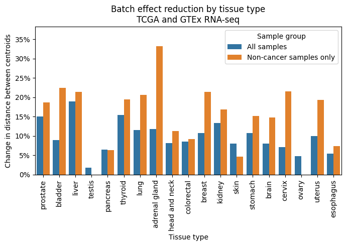
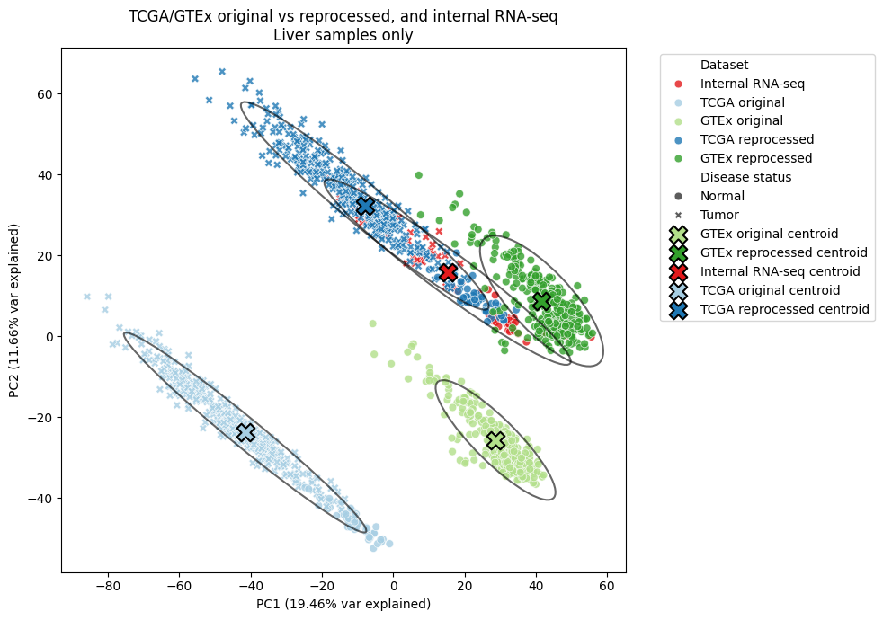
In the liver, where we have the most internal RNA-seq data, all three data sources were much closer in PC-space after re-processing. I’m particularly happy about this result, as it means our internally-generated data can be compared with these external sources more reliably.
References
- Arora, S., Pattwell, S. S., Holland, E. C. & Bolouri, H. Variability in estimated gene expression among commonly used RNA-seq pipelines. Sci Rep10, 2734 (2020).
- Wang, Q. et al. Unifying cancer and normal RNA sequencing data from different sources. Sci Data5, 180061 (2018).