Rare transmission of commensal and pathogenic bacteria in the gut microbiome of hospitalized adults (1)

My final project with the Bhatt Lab is now published! You can find the open access text at Nature Communications. I’m excited to bring this chapter of my research career to a close. The paper contains the full scientific results; here I’ll detail some of the journey and challenges along the way.

Hot off the success of my previous work studying mother-infant transmission of phages in the microbiome, I was eager to characterize other examples transmission between the microbiome of humans. While mother-infant transmission of both bacteria and phages was now understood, microbiome transmission between adults was less clear. There were some hints of it happening in the literature, but nobody had fully characterized the phenomenon at a genomic level of detail that I believed. I’m also not counting FMT as transmission here – while it certainly results in the transfer of microbiome components from donor to recipient, I was more interested in characterizing how this phenomenon happened naturally.

In our lab, we have a stool sample biobank from patients undergoing hematopoietic cell transplantation (HCT). We’ve been collecting weekly stool samples from patients undergoing transplant at Stanford Hospital, and to date we have thousands of samples from about one thousand patients. HCT patients are prime candidates to study gut-gut bacterial transmission, due to a few key factors:

  1. Long hospital stays. The conditioning, transplant and recovery process can leave a patient hospitalized for up to months at a time. The long stays provide many opportunities for transmission to occur and many longitudinal samples for us to analyze.
  2. Roommates when recovering from transplant. At Stanford Hospital, patients were placed in double occupancy rooms when there were not active contact precautions. These periods of roommate overlap could provide an increased chance for patient-patient transmission.
  3. Frequent antibiotic use. HCT patients are prescribed antibiotics both prophylactically and in response to infection. These antibiotics kill the natural colonizers of the gut microbiome, allowing antibiotic resistant pathogens to dominate, which may be more likely to be transmitted between patients. Antibiotic use may also empty the niche occupied by certain bacteria and make it more likely for new colonizers to engraft long-term.
  4. High burden of infection. HCT patients frequently have potentially life-threatening infections, and the causal bacteria can originate in the gut microbiome. However, it’s currently unknown where these antibiotic resistant bacteria originate from in the first place. Could transmission from another patient be responsible?

As we thought more about the cases of infection that were caused by gut-bloodstream transmission, we identified three possibilities:

  1. The microbes existed in the patient’s microbiome prior to entering the hospital for HCT. Then, due to antibiotic use and chemotherapy, these microbes could come to dominate the gut community.
  2. Patients acquired the microbe from the hospital environment. Many of the pathogens we’re interested in are Hospital Acquired Infections (HAIs) and known to persist for long periods of time on on hospital surfaces, in sinks, etc.
  3. Patients acquired the microbe via transmission from another patient. This was the most interesting possibility to us, as it would indicate direct gut-gut transmission.

While it’s likely that all three are responsible to some degree, finding evidence for (3) would have been the most interesting to us. Identifying patient-patient microbiome transmission would be both a slam dunk for my research, and would potentially help prevent infections in this patient population. With the clear goal in mind, I opened the door of the -80 freezer to pull out the hundreds of stool samples I would need to analyze…

More to come in part 2!


Large-scale bioinformatics in the cloud with GCP, Kubernetes and Snakemake

I recently finished a large metagenomics sequencing experiment – 96 10X Genomics linked read libraries sequenced across 25 lanes on a HiSeq4000. This was around 2TB of raw data (compressed fastqs). I’ll go into more detail about the project and data in another post, but here I’m just going to talk about processing the raw data.

We’re lucky to have a large compute cluster at Stanford for our every day work. This is shared with other labs and has a priority system for managing compute resouces. It’s fine for most tasks, but not up to the scope of this current project. 2TB of raw data may not be “big” in the scale of what places like the Broad deal with on a daily basis, but it’s definitely the largest single sequencing experiment I and our lab has done. To solve this, we had to move… TO THE CLOUD!

By utilizing cloud compute, I can easily scale the compute resources to the problem at hand. Total cost is the same if you use 1 cpu for 100 hours or 100 cpus for 1 hour… so I will parallelize this as much as possible to minimize the time taken to process the data. We use Google Cloud Comptue (GCP) for bioinformatics, but you can do something similar with Amazon’s or Microsoft’s cloud compute, too. I used ideas from this blog post to port the Bhatt lab metagenomics workflows to GCP.

Step 0: Install the GCP SDK, Configure a storage bucket.

Install the GCP SDK to manage your instances and connect to them from the command line. Create a storage bucket for data from this project – this can be done from the GCP console on the web. Then, set up authentication as described here.

Step 1: Download the raw data

Our sequencing provider provides raw data via an FTP server. I downloaded all the data from the FTP server and uploaded it to the storage bucket using the gsutil rsync command. Note that any reference databases (human genome for removing human reads, for example) need to be in the cloud too.

Step 2: Configure your workflow.

I’m going to assume you already have a snakemake workflow that works with local compute. Here, I’ll show how to transform it to work with cloud compute. I’ll use the workflow to run the 10X Genomics longranger basic program and deinterleave reads as an example. This takes in a number of samples with forward and reverse paired end reads, and outputs the processed reads as gzipped files.

The first lines import the cloud compute packages, define your storage bucket, and search for all samples matching a specific name on the cloud.

from os.path import join
from snakemake.remote.GS import RemoteProvider as GSRemoteProvider
GS = GSRemoteProvider()
GS_PREFIX = "YOUR_BUCKET_HERE"
samples, *_ = GS.glob_wildcards(GS_PREFIX + '/raw_data_renamed/{sample}_S1_L001_R1_001.fastq.gz')
print(samples)

The rest of the workflow just has a few modifications. Note that Snakemake automatically takes care of remote input and output file locations. However, you need to add the ‘GS_PREFIX’ when specifying folders as parameters. Also, if output files aren’t explicitly specified, they don’t get uploaded to remote storage. Note the use of a singularity image for the longranger rule, which automatically gets pulled on the compute node and has the longranger program in it. pigz isn’t available on the cloud compute nodes by default, so the deinterleave rule has a simple conda environment that specifies installing pigz. The full pipeline (and others) can be found at the Bhatt lab github.

rule all:
    input:
        expand('barcoded_fastq_deinterleaved/{sample}_1.fq.gz', sample=samples)

rule longranger:
    input: 
        r1 = 'raw_data_renamed/{sample}_S1_L001_R1_001.fastq.gz',
        r2 = 'raw_data_renamed/{sample}_S1_L001_R2_001.fastq.gz'
    output: 'barcoded_fastq/{sample}_barcoded.fastq.gz'
    singularity: "docker://biocontainers/longranger:v2.2.2_cv2"
    threads: 15
    resources:
        mem=30,
        time=12
    params:
        fq_dir = join(GS_PREFIX, 'raw_data_renamed'),
        outdir = join(GS_PREFIX, '{sample}'),
    shell: """
        longranger basic --fastqs {params.fq_dir} --id {wildcards.sample} \
            --sample {wildcards.sample} --disable-ui --localcores={threads}
        mv {wildcards.sample}/outs/barcoded.fastq.gz {output}
    """

rule deinterleave:
    input:
        rules.longranger.output
    output:
        r1 = 'barcoded_fastq_deinterleaved/{sample}_1.fq.gz',
        r2 = 'barcoded_fastq_deinterleaved/{sample}_2.fq.gz'
    conda: "envs/pigz.yaml"
    threads: 7
    resources: 
        mem=8,
        time=12
    shell: """
        # code inspired by https://gist.github.com/3521724
        zcat {input} | paste - - - - - - - -  | tee >(cut -f 1-4 | tr "\t" "\n" |
            pigz --best --processes {threads} > {output.r1}) | \
            cut -f 5-8 | tr "\t" "\n" | pigz --best --processes {threads} > {output.r2}
    """

Now that the input files and workflow are ready to go, we need to set up our compute cluster. Here I use a Kubernetes cluster which has several attractive features, such as autoscaling of compute resources to demand.

A few points of terminology that will be useful:

  • A cluster contains (potentially multiple) node pools.
  • A node pool contains multiple nodes of the same type
  • A node is the basic compute unit, that can contain multiple cpus
  • A pod (as in a pod of whales) is the unit or job of deployed compute on a node

To start a cluster, run a command like this. Change the parameters to the type of machine that you need. The last line gets credentials for job submission. This starts with a single node, and enables autoscaling up to 96 nodes.

export CLUSTER_NAME="snakemake-cluster-big"
export ZONE="us-west1-b"
gcloud container clusters create $CLUSTER_NAME \
    --zone=$ZONE --num-nodes=1 \
    --machine-type="n1-standard-8" \
    --scopes storage-rw \
    --image-type=UBUNTU \
    --disk-size=500GB \
    --enable-autoscaling \
    --max-nodes=96 \
    --min-nodes=0
gcloud container clusters get-credentials --zone=$ZONE $CLUSTER_NAME

For jobs with different compute needs, you can add a new node pool like so. I used two different node pools, with 8 core nodes for preprocessing the sequencing data and aligning against the human genome, and 16 core nodes for assembly. You could also create additional high memory pools, GPU pools, etc depending on your needs. Ensure new node pools are set with --scopes storage-rw to allow writing to buckets!

gcloud container node-pools create pool2 \
    --cluster $CLUSTER_NAME \
    --zone=$ZONE --num-nodes=1 \
    --machine-type="n1-standard-16" \
    --scopes storage-rw \
    --image-type=UBUNTU \
    --disk-size=500GB \
    --enable-autoscaling \
    --max-nodes=96 \
    --min-nodes=0

When you are finished with the workflow, shut down the cluster with this command. Or let autoscaling slowly move the number of machines down to zero.

gcloud container clusters delete --zone $ZONE $CLUSTER_NAME

To run the snakemake pipeline and submit jobs to the Kubernetes cluster, use a command like this:

snakemake -s 10x_longranger.snakefile --default-remote-provider GS \
    --default-remote-prefix YOUR_BUCKET_HERE --use-singularity \
    -j 99999 --use-conda --nolock --kubernetes

Add the name of your bucket prefix. The ‘-j’ here allows (mostly) unlimited jobs to be scheduled simultaneously.

Each job will be assigned to a node with available resources. You can monitor the progress and logs with the commands shown as output. Kubernetes autoscaling takes care of provisioning new nodes when more capacity is needed, and removes nodes from the pool when they’re not needed any more. There is some lag for removing nodes, so beware of the extra costs.

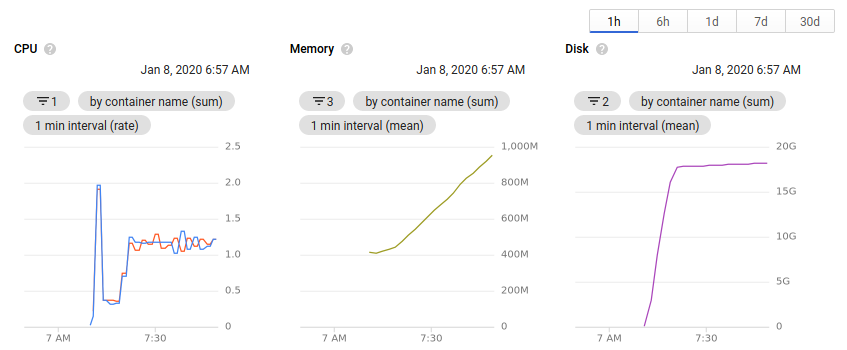
While the cluster is running, you can view the number of nodes allocated and the available resources all within the browser. Clicking on an individual node or pod will give an overview of the resource usage over time.

Useful things I learned while working on this project

  • Use docker and singularity images where possible. In cases where multiple tools were needed, a simple conda environment does the trick.
  • The container image type must be set to Ubuntu (see above) for singularity images to correctly work on the cluster.
  • It’s important to define memory requirements much more rigorously when working on the cloud. Compared to our local cluster, standard GCP nodes have much less memory. I had to go through each pipeline and define an appropriate amount of memory for each job, otherwise they wouldn’t schedule from Kubernetes, or would be killed when they exceeded the limit.
  • You can only reliably use n-1 cores on each node in a Kubernetes cluster. There’s always some processes running on a node in the background, and Kubernetes will not scale an excess of 100% cpu. The threads parameter in snakemake is an integer. Combine these two things and you can only really use 7 cores on an 8-core machine. If anyone has a way around this, please let me know!
  • When defining input and output files, you need to be much more specific. When working on the cluster, I would just specify a single output file out of many for a program, and could trust that the others would be there when I needed them. But when working with remote files, the outputs need to be specified explicitly to get uploaded to the bucket. Maybe this could be fixed with a call to directory() in the output files, but I haven’t tried that yet.
  • Snakemake automatically takes care of remote files in inputs and outputs, but paths specified in the params: section do not automatically get converted. I use paths here for specifying an output directory when a program asks for it. You need to add the GS_PREFIX to paths to ensure they’re remote. Again, might be fixed with a directory() call in the output files.
  • I haven’t been able to get configuration yaml files to work well in the cloud. I’ve just been specifying configuration parameters in the snakefile or on the command line.

Transmission of crAsspahge in the microbiome

Update! This work has been published in Nature Communications.
Siranosian, B.A., Tamburini, F.B., Sherlock, G. et al. Acquisition, transmission and strain diversity of human gut-colonizing crAss-like phages. Nat Commun 11, 280 (2020). https://doi.org/10.1038/s41467-019-14103-3

Big questions in the microbiome field surround the topic of microbiome acquisition. Where do we get our first microbes from? What determines the microbes that colonize our guts form birth, and how do they change over time? What short and long term impacts do these microbes have on the immune system, allergies or diseases? What impact do delivery mode and breastfeeding have on the infant microbiome?

A key finding from the work was that mothers and infants often share identical or nearly identical crAssphage sequences, suggesting direct vertical transmission. Also, I love heatmaps.

As you might expect, a major source for microbes colonizing the infant gut is immediate family members, and the mother is thought to be the major source. Thanks to foundational studies by Bäckhed, Feretti, Yassour and others (references below), we now know that infants often acquire the primary bacterial strain from the mother’s microbiome. These microbes can have beneficial capabilities for the infant, such as the ability to digest human milk oligosaccharides, a key source of nutrients in breast milk.

The microbiome isn’t just bacteria – phages (along with fungi and archaea to a smaller extent) play key roles. Phages are viruses that predate on bacteria, depleting certain populations and exchanging genes among the bacteria they infect. Interestingly, phages were previously shown to display different inheritance patterns than bacteria, remaining individual-specific between family members and even twins (Reyes et al. 2010). CrAss-like phages are the most prevalent and abundant group of phages colonizing the human gut, and our lab was interested in the inheritance patterns of these phages.

We examined publicly available shotgun gut metagenomic datasets from two studies (Yassour et al. 2018, Bäckhed et al. 2015), containing 134 mother-infant pairs sampled extensively through the first year of life. In contrast to what has been observed for other members of the gut virome, we observed many putative transmission events of a crAss-like phage from mother to infant. The key takeaways from our research are summarized below. You can also refer my poster from the Cold Spring Harbor Microbiome meeting for the figures supporting these points. We hope to have a new preprint (and hopefully a publication) on this research out soon!

  1. CrAssphage is not detected in infant microbiomes at birth, increases in prevalence with age, but doesn’t reach the level of adults by 12 months of age.
  2. Mothers and infants share nearly identical crAssphage genomes in 40% of cases, suggesting vertical transmission.
  3. Infants have reduced crAssphage strain diversity and typically acquire the mother’s dominant strain upon transmission.
  4. Strain diversity is mostly the result of neutral genetic variation, but infants have more nonsynonymous multiallelic sites than mothers.
  5. Strain diversity varies across the genome, and tail fiber genes are enriched for strain diversity with nonsynonymous variants.
  6. These findings extend to crAss-like phages. Vaginally born infants are more likely to have crAss-lke phages than those born via C-section.

References
1. Reyes, A. et al. Viruses in the faecal microbiota of monozygotic twins and their mothers. Nature 466, 334–338 (2010).
2. Yassour, M. et al. Strain-Level Analysis of Mother-to-Child Bacterial Transmission during the First Few Months of Life. Cell Host & Microbe 24, 146-154.e4 (2018).
3. Bäckhed, F. et al. Dynamics and Stabilization of the Human Gut Microbiome during the First Year of Life. Cell Host & Microbe 17, 690–703 (2015).
4. Ferretti, P. et al. Mother-to-Infant Microbial Transmission from Different Body Sites Shapes the Developing Infant Gut Microbiome. Cell Host & Microbe 24, 133-145.e5 (2018).

What is crAssphage?

CrAssphage is a like mystery novel full of surprises. First described in 2014 by Dutilh et al., crAssphage acquired it’s (rather unfortunate, given that it colonizes the human intestine) name from the “Cross-Assembly” bioinformatics method used to characterize it. CrAssphage interests me because it’s prevalent in up to 70% of human gut microbiomes, and can make up the majority of viral sequencing reads in a metagenomics experiment. This makes it the most successful single entity colonizing human microbiomes. However, no health impacts have been demonstrated from having crAssphage in your gut – several studies (Edwards et al. 2019) have turned up negative.

Electron micrograph of a representative crAssphage, from Shkoporov et al. (2018). This phage is a member of the Podoviridae family and infects Bacteroides Intestinalis.

CrAssphage was always suspected to predate on species of the Bacteroides genus based on evidence from abundance correlation and CRISPR spacers. However, the phage proved difficult to isolate and culture. It wasn’t until recently that a crAssphage was confirmed to infect Bacteroides intestinalis (Shakoporov et al. 2018). They also got a great TEM image of the phage! With crAssphage successfully cultured in the lab, scientists have begun to answer fundamental questions about its biology. The phage appears to have a narrow host range, infecting a single B. intestinalis strain and not others or other species. The life cycle of the phage was puzzling:

“We can conclude that the virus probably causes a successful lytic infection with a size of progeny per capita higher than 2.5 in a subset of infected cells (giving rise to a false overall burst size of ~2.5), and also enters an alternative interaction (pseudolysogeny, dormant, carrier state, etc.) with some or all of the remaining cells. Overall, this allows both bacteriophage and host to co-exist in a stable interaction over prolonged passages. The nature of this interaction warrants further investigation.” (Shakoporov et al. 2018)

Further investigation showed that crAssphage is one member of an extensive family of “crAss-like” phages colonizing the human gut. Guerin et al. (2018) proposed a classification system for these phages, which contains 4 subfamilies (Alpha, Beta, Delta and Gamma) and 10 clusters. The first described “prototypical crAssphage” belongs to the Alpha subfamily, cluster 1. It struck me how diverse these phages are – different families are less than 20% identical at the protein level! When all crAss-like phages are considered, it’s estimated that up to 100% of individuals cary at least one crAss-like phage, and most people cary more than one.

Given the high prevalence of crAss-like phages and their specificity for the human gut, they do have an interesting use as a tracking device for human sewage. DNA from crAss-like phages can be used to track waste contamination into water, for example (Stachler et al. 2018). In a similar vein, our lab has used crAss-like phages to better understand how microbes are transmitted from mothers to newborn infants. The small genome sizes (around 100kb) and high prevalence/abundance make these phages good tools for doing strain-resolved metagenomics. Trust me, you’d much rather do genomic assembly and variant calling on a 100kb phage genome than a 3Mb bacterial genome!

Research into crAss-like phages is just beginning, and I’m excited to see what’s uncovered in the future. What are the hosts of the various phage clusters? How do these phages influence gut bacterial communities? Do crAss-like phages exclude other closely related phages from colonizing their niches, leading to the low strain diversity we observe? Can crAss-like phgaes be used to engineer bacteria in the microbiome, delivering precise genetic payloads? This final question in the most interesting to me, given that crAss-like phages seem relatively benign to humans, yet incredibly capable of infecting our microbes.

References
1.Dutilh, B. E. et al. A highly abundant bacteriophage discovered in the unknown sequences of human faecal metagenomes. Nature Communications 5, 4498 (2014).
2.Edwards, R. A. et al. Global phylogeography and ancient evolution of the widespread human gut virus crAssphage. Nature Microbiology 1 (2019). doi:10.1038/s41564-019-0494-6
3.Guerin, E. et al. Biology and Taxonomy of crAss-like Bacteriophages, the Most Abundant Virus in the Human Gut. Cell Host & Microbe 0, (2018).
4.Shkoporov, A. N. et al. ΦCrAss001 represents the most abundant bacteriophage family in the human gut and infects Bacteroides intestinalis. Nature Communications 9, 4781 (2018).
5.Stachler, E., Akyon, B., de Carvalho, N. A., Ference, C. & Bibby, K. Correlation of crAssphage qPCR Markers with Culturable and Molecular Indicators of Human Fecal Pollution in an Impacted Urban Watershed. Environ. Sci. Technol. 52, 7505–7512 (2018).

Metagenome Assembled Genomes enhance short read classification

In the microbiome field we struggle with the fact that reference databases are (sometimes woefully) incomplete. Many gut microbes are difficult to isolate and culture in the lab or simply haven’t been sampled frequently enough for us to study. The problem is especially bad when studying microbiome samples from non-Western individuals.

To subvert the difficulty in culturing new organisms, researchers try to create new reference genomes directly from metagenomic samples. This typically uses metagenomic assembly and binning. Although you most likely end up with a sequence that isn’t entirely representative of the organism, these Metagenome Assembled Genomes (MAGs) are a good place to start. They provide new reference genomes for classification and association testing, and start to explain what’s in the microbial “dark matter” from a metagenomic sample.

2019 has been a good year for MAGs. Three high profile papers highlighting MAG collections were published in the last few months[1,2,3]. The main idea in each of them was similar – gather a ton of microbiome data, assemble and bin contigs, filter for quality and undiscovered genomes, do some analysis of the results. My main complaint about all three papers is that they use reduced quality metrics, not following the standards set in Bowers et al. (2017). They rarely find 16S rRNA sequences in genomes called “high quality,” for example.

Comparing the datasets, methods, and results from the three MAG studies. This table was compiled by Yiran Liu during her Bhatt lab rotation.

After reading the three MAG papers, Nayfach et al. (2019) is my favortie. His paper does the most analysis into what these new genomes _mean_, including a great finding presented in Figure 4. These new references assembled from metagenomes can help explain why previous studies looking for associations between the microbiome and disease have come up negative. This can also help explain why microbiome studies have been difficult to replicate. If a significant association is hiding in these previously unclassified genomes, a false positive association could easily look significant because everything is tested with relative abundance.

In the Bhatt lab, we were interested in using these new MAG databases to improve classification rates in some samples from South African individuals. First we had to build a Kraken2 database for the MAG collections. If you’re interested in how to do this, I have an instructional example over at the Kraken2 classification GitHub. For samples from Western individuals, the classification percentages don’t increase much with MAG databases, in line with what we would expect. For samples from South African individuals, the gain is sizeable. We see the greatest increase in classification percentages by using the Almeida et al. (2019) genomes. This collection is the largest, and may represent a sensitivity/specificity tradeoff. The percentages represented below for MAG databases are calculated as the total classifies percentages when the unclassified reads from our standard Kraken2 database are run through the MAG database.

Classification percentages on samples from Western individuals. We’re already doing pretty good without the MAG database.

Classification percentages on non-Western individuals. MAGs add a good amount here. Data collected and processed by Fiona Tamburini.


References
1.Nayfach, S., Shi, Z. J., Seshadri, R., Pollard, K. S. & Kyrpides, N. C. New insights from uncultivated genomes of the global human gut microbiome. Nature 568, 505 (2019).
2.Pasolli, E. et al. Extensive Unexplored Human Microbiome Diversity Revealed by Over 150,000 Genomes from Metagenomes Spanning Age, Geography, and Lifestyle. Cell 0, (2019).
3.Almeida, A. et al. A new genomic blueprint of the human gut microbiota. Nature 1 (2019). doi:10.1038/s41586-019-0965-1
4.Bowers, R. M. et al. Minimum information about a single amplified genome (MISAG) and a metagenome-assembled genome (MIMAG) of bacteria and archaea. Nature Biotechnology 35, 725–731 (2017).

Short read classification with Kraken2

After sequencing a community of bacteria, phages, fungi and other organisms in a microbiome experiment, the first question we tend to ask is “What’s in my sample?” This task, known as metagenomic classification, aims to assign a classification to each sequencing read from your experiment. My favorite program to answer this question is Kraken2, although it’s not the only tool for the job. Others like Centrifuge and even Blast have their merits. In our lab, we’ve found Kraken2 to be very sensitive with our custom database, and very fast to run across millions or sequencing reads. Kraken2 is best paired with Bracken for estimation of relative abundance of organisms in your sample.

I’ve built a custom Kraken2 database that’s much more expansive than the default recommended by the authors. First, it uses Genbank instead of RefSeq. It also uses genomes assembled to “chromosome” or “scaffold” quality, in addition to the default “complete genome.” The default database misses some key organisms that often show up in our experiments, like Bacteroides intestinalis. This is not noted in the documentation anywhere, and is unacceptable in my mind. But it’s a key reminder that a classification program is only as good as the database it uses. The cost for the expanded custom database is greatly increased memory usage and increased classification time. Instructions for building a database this way are over at my Kraken2 GitHub.

With the custom database, we often see classification percentages as high as 95% for western human stool metagenomic datasets. The percentages are lower in non-western guts, and lower still for mice

Read classification percentages with Kraken2 and a custom Genbank database. We’re best at samples from Western individuals, but much worse at samples from African individuals (Soweto, Agincourt and Tanzania). This is due to biases in our reference databases.

With the high sensitivity of Kraken/Bracken comes a tradeoff in specificity. For example, we’re often shown that a sample contains small proportions of many closely related species. Are all of these actually present in the sample? Likely not. These species probably have closely related genomes, and reads mapping to homologous regions can’t be distinguished between them. When Bracken redistributes reads back down the taxonomy tree, they aggregate at all the similar species. This means it’s sometimes better to work at the genus level, even though most of our reads can be classified down to a species. This problem could be alleviated by manual database curation, but who has time for that?

Are all these Porphyromonadacae actually in your sample? Doubt it.

Also at the Kraken2 GitHub is a pipeline written in Snakemake and that takes advantage of Singularity containerization. This allows you to run metagenomic classification on many samples, process the results and generate informative figures all with a single command! The output is taxonomic classification matrices at each level (species, genus, etc), taxonomic barplots, dimensionality reduction plots, and more. You can also specify groups of samples to test for statistical differences in the populations of microbes.

Taxonomic barplot at the species level of an infant microbiome during the first three months of life, data from Yassour et al. (2018). You can see the characteristic Biffidobacterium in the early samples, as well as some human reads that escaped removal in preprocessing of these data.


Principal coordinates analysis plot of microbiome samples from mothers and infants from two families. Adults appear similar to each other, while the infants from two families remain distinct.

I’m actively maintaining the Kraken2 repository and will add new features upon request. Up next: compositional data analysis of the classification results.

References:
Wood, D. E. & Salzberg, S. L. Kraken: ultrafast metagenomic sequence classification using exact alignments. Genome Biol. 15, R46 (2014).
Yassour, M. et al. Strain-Level Analysis of Mother-to-Child Bacterial Transmission during the First Few Months of Life. Cell Host & Microbe 24, 146-154.e4 (2018).

Joining the Bhatt lab

My third lab rotation in my first year at Stanford took a different path than most of my previous experience. I came to Stanford expecting to research chromatin structure – 3D conformation, gene expression, functional consequences. My past post history shows this interest undoubtedly, and people in my class even referred to me as the “Chromatin Structure Guy.” However, approaching my third quarter lab rotation I was looking for something a little different. Rotations are a great time to try something new and a research area you’re not experienced in.

I decided to rotate in Dr. Ami Bhatt’s lab. She’s an MD/PhD broadly interested in the human microbiome and its influence on human health. With dual appointments in the departments of Genetics and Hematology, she has great clinical research projects as well. Plus, the lab does interesting method development on new sequencing technologies, DNA extraction protocols and bioinformatics techniques. The microbiome research area is rapidly expanding, as gut microbial composition has been shown to play a role in a huge range of human health conditions, from psychiatry to cancer immunotherapy response. “What a great chance to work on something new for a few months?” I told myself. “I can always go back to a chromatin lab after the rotation is over”

I never thought I would find the research so interesting, and like the lab so much.

So, I joined a poop lab. I’ll let that one sink in. We work with stool samples so much that we have to make light of it. Stool jokes are commonplace, even encouraged, in lab meeting presentations. Everyone in the lab is required to make their own “poo-moji” after they join.

My poo-moji. What a likeness!

I did my inaugural microbial DNA extraction from stool samples last week. I was expecting worse; it didn’t smell nearly as bad as I expected. Still, running this protocol always has me thinking about the potential for things to end very badly:

  1. Place frozen stool in buffer
  2. Heat to 85 degrees C
  3. Vortex violently for 1 minute
  4. ….

Yes, we have tubes full of liquid poo, heated to nearly boiling temperature, shaking about violently on the bench! You can bet I made sure those caps were on tight.

Jokes aside, my interest in this field continues to grow the more I read about the microbiome. As a start, here are some of the genomics and methods topics I find interesting at the moment:

  • Metagenomic binning. Metagenomics often centers around working on organisms without a reference genome – maybe the organism has never been sequenced before, or it has diverged so much from a reference that it’s essentially useless. Without aligning to a reference sequence, how can we cluster contigs assembled from a metagenomic sequencing experiment such that a cluster likely represents a single organism?
  • Linked reads, which provide long-range information to a typical short read genome sequencing dataset. They can massively aid in assembly and recovery of complete genomes from a metagenome.
  • k-mer analysis. How can short sequences of DNA be used to quickly classify a sequencing read, or determine if a particular organism is in a metagenomic sample? This hearkens to some research I did in undergrad on tetranucleotide usage in bacteriophage genomes. Maybe this field isn’t too foreign after all!

On the biological side, there’s almost too much to list. It seems like the microbiome plays a role in every bodily process involving metabolism or the immune system. Yes, that’s basically everything. For a start:

  • Establishment of the microbiome. A newborn’s immune system has to tolerate microbes in the gut without mounting an immune overreaction, but also has to prevent pathogenic organisms from taking hold. The delicate interplay between these processes, and how the balance is maintained, is very interesting to me.
  • The microbiome’s role in cancer immunotherapy. Mice without a microbiome respond poorly to cancer immunotherapy, and the efficacy of treatment can reliably be altered with antibiotics. Although researchers have shown certain bacterial groups are associated with better or worse outcomes in patients, I’d really like to move this research beyond correlative analysis.
  • Fecal microbial transplants (FMT) for Clostridium difficile infection. FMT is one of the most effective ways to treat C. difficile, a infection typically acquired in hospitals and nursing homes that costs tens of thousands of lives per year. Transferring microbes from a healthy donor to a infected patient is one of the best treatments, but we’re not sure of the specifics of how it works. Which microbes are necessary and sufficient to displace C. diff? Attempts to engineer a curative community of bacteria by selecting individual strains have failed, can we do better by comparing simplified microbial communities from a stool donor?

Honestly, it feels great to be done with rotations and to have a decided lab “home.” With the first year of graduate school almost over, I can now spend my time in more focused research and avoid classes for the time being. More microbiome posts to come soon!