Accelerated computing is the future of genomics

“We’re out of storage, and we’re out of compute.” I’ll never forget the 2016 Broad Institute Cancer Program meeting where Eric Banks, senior director of the Data Sciences Platform, showed the audience how much genomic data the Broad was generating. The exponential curve was plotted against the current capacity of the on-premises compute cluster –  the time until intersection of the curves could be measured in months. In fact, we were generating data even faster than we could add new storage drives. This meeting sparked the Broad’s move to the cloud for the majority of data storage and compute.

While moving to the cloud may have been the simple answer seven years ago, it’s not a catch-all solution today. Genome sequencing costs have dropped precipitously, and newer high-content assays like single-cell sequencing and spatial transcriptomics are being developed every day. Storing and processing all these data requires a massive amount of resources, and a cloud bill to match (even if you’re trying to do the analysis on the cheap). We need new, more efficient ways to process, store and transfer genomic data. Enter accelerated computing.

Accelerated computing, the use of special-purpose hardware for specific computational tasks, can help solve many of the problems facing genomics today. Using Graphical Processing Units (GPUs) and similar hardware, these custom-developed algorithms can reduce the time needed to run an analysis by a factor of 10 to 100. This great reduction in compute time has paved the way for more efficient data processing and real-time analysis in clinical genomics.

In this series, I’ll cover three topics related to accelerated computing in genomics:

  • An overview of the basics of accelerated computing, the popular tools, and the companies developing them (this post).
  • Practical considerations. How can you use these tools today? (coming soon)
  • Algorithmic details. How do accelerated tools work to drastically decrease the runtime of common tasks? What problems in genomics are amenable to acceleration? (a future post)

Accelerated computing is a general term describing the use of specialized hardware to speed up a certain computation. Commonly used hardware in the genomics space includes:

  • Graphical Processing Units (GPUs)
  • Field Programmable Gate Arrays (FPGAs)
  • Application-specific integrated circuits (ASICs)
  • Tensor Processing Units (TPUs)

While Central Processing Units (CPUs) excel at general-purpose tasks, they lack the ability to run many computations in parallel. GPUs are the opposite. While they were originally developed for video game rendering, GPUs excel at parallel computations. They can have thousands of processor cores, each capable of running a calculation in parallel. Accelerated computing takes advantage of each hardware type for the tasks it is best at. Control functionality and single-threaded work is left to the CPU, and parallelizable computations are done on the GPU. NVIDIA Clara Parabricks leads the way in GPU-accelerated genomics.

FPGAs allow for the hardware to be reconfigured on the fly to run a specific algorithm. They are used in the Illumina DRAGEN tools I’ll cover later. ASICs are less common. They have a fixed configuration and perform a limited set of functions, so they’re best used in very specific settings, like controlling the pores on an Oxford Nanopore MinION. TPUs are used in training ML models to interpret genomic data, but not in the processing of the data directly.

While GPU-based training of deep learning models is standard and supported by key libraries in the ecosystem, in traditional genomics fashion, the field is 5-10 years behind other industries. We are starting to see GPU-based genomics tools being released, but they’re closed source and still gaining traction. By contrast, PyTorch, a popular open source machine learning framework, was released in 2016! My prediction is that accelerated tools will become standard in genomics as well, but we need a lot of work to get there.

How can I use hardware acceleration in genomics today?

Your best bet is to use one of these developed toolkits. If you don’t have access to a machine with GPUs or FPGAs, they can be rented from AWS or GCP for a low hourly fee.

NVIDIA Clara Parabricks: GPU-accelerated alignment, variant calling, and RNA-seq

NVIDIA’s entry into GPU-accelerated genomics is the result of the 2019 acquisition of the software startup Parabricks. NVIDIA first released the software as closed access, but with the version 4.0 release in 2022, anyone can download the docker container and run the software. Parabricks runs on most modern NVIDIA GPUs and accelerates alignment of DNA and RNA-seq data, variant calling, and other time-intensive processes by up to 80x (using a multi-GPU machine). Parabricks was designed as a drop-in replacement for common tools like GATK, and is guaranteed to produce an identical output as certain GATK versions. Running the software is simple, all you have to do is pull the docker container at nvcr.io/nvidia/clara/clara-parabricks:4.0.0-1 and run one of the command line tools.

The strengths of Parabricks lie in its ease of use, wide applicability, and cost effectiveness. GPUs are everywhere: on the cloud, in gaming PCs, and in servers used for ML/AI training. The docker container is available for anyone to try for free, without a license or multiple sales calls. Parabricks also attempts to automate some processes that may have been spread across multiple tools in the past: alignments are always  coordinate-sorted, for example.

The weaknesses of Parabricks come down to the limited functionality and lack of integration, at least compared to DRAGEN. Parabricks doesn’t have the advanced functionality of DRAGEN for tasks like single-cell sequencing and star-allele calling for pharmacogenomics. And you obviously can’t buy an Illumina sequencer with a competitor’s hardware and software in it!

Illumina DRAGEN: FPGA-accelerated Bio-IT platform

Illumina recognized the challenges in storage and processing of genomic data early, and acquired Edico Genome and the DRAGEN Bio-IT platform in 2018 to architect a solution. DRAGEN uses FPGAs to speed up generation of FASTQ files, alignment, variant calling, and many other processes. In addition to a standard GATK implementation, DRAGEN designed their own variant calling algorithms which have won two out of three of the Precision FDA Truth Challenge V2 Illumina categories. DRAGEN also provides new algorithms for accelerated single-cell genomics, star-allele calling, and other processes.

The strengths of DRAGEN lie in the tight integration with Illumina products. You can buy an Illumina sequencer with a DRAGEN server built in, so that everything up to variant calling can be completed on the sequencer. This means the large raw data files never have to be transferred to the cloud or elsewhere, saving on storage costs (as long as you don’t need the raw data for backup or compliance purposes). The accuracy, speed, and continued improvement of the algorithms are another key advantage.

The weaknesses of DRAGEN come with the costs of using the software. Since Illumina doesn’t benefit from the purchase of FPGAs, they charge a LOT for the DRAGEN license. In fact, the license cost is 80% of the total cost when running DRAGEN on the cloud! This deters researchers in academia and lower-resourced companies from using DRAGEN, and may push them to a free alternative instead.

Nanopore and PacBio sequencers: accelerated computing right under the hood

Oxford Nanopore uses hardware acceleration at multiple places in their long-read sequencers. Pores on the flowcells are controlled by ASICs, and the more advanced multi-flowcell workstations use GPUs to accelerate data analysis. The Nanopore Promethion comes with 4 NVIDIA A100 GPUs, for example. PacBio’s new Revio sequencer has a similar arrangement, with on-board GPUs to speed up the processing of raw data. While Nanopore and PacBio sequencers both take advantage of hardware acceleration, there’s much less direct interaction with the algorithms, compared to the user-facing toolkits above.

Where’s the PyTorch of genomics?

All of the accelerated genomics toolkits I’ve talked about today are being developed closed-source by publicly traded companies. That’s great for efficient development of high-performance code, but it shuts out the community of developers in academia or low-resource industries that might use and contribute to your code. NVIDIA had GenomeWorks, but that hasn’t seen a commit in a year and a half. Some other groups are repurposing GPU-accelerated Python libraries for single-cell analysis.

If you’re working on an open-source GPU genomics toolkit, I’d love to hear about it.

One final thought: the story of how GPUs transitioned from gaming devices to general-purpose compute accelerators is both fascinating and entertaining. It all started with a quantum chemistry professor at Stanford buying NVIDIA gaming cards in 2006 and hacking them to do the computation he needed. Acquired has a great podcast on the topic.

Deep learning to understand and predict single-cell chromatin structure

In my last post, I described how to simulate ensembles of structures representing the 3D conformation of chromatin inside the nucleus. Now, I’m going to describe some of my research to use deep learning methods, particularly an autoencoder/decoder, to do some interesting things with this data:

  • Cluster structures from individual cells. The autoencoder should be able to learn a reduced-dimensionality representation of the data that will allow better clustering.
  • Reduce noise in experimental data.
  • Predict missing points in experimental data.

Something I learned early on rotating in the Kundaje lab at Stanford is that deep learning methods might seem domain specific at first. However, if you can translate your data and question into a problem that has already been studied by other researchers, you can benefit from their work and expertise. For example, if I want to use deep learning methods on 3D chromatin structure data, that will be difficult because few methods have been developed to work on point coordinates in 3D. However, the field of image processing has a wealth of deep learning research. A 3D structure can easily be represented by a 2D distance or contact map – essentially a grayscale image. By translating a 3D structure problem into a 2D image problem, we can use many of the methods and techniques already developed for image processing.

Autoencoders and decoders

The primary model I’m going to use is a convolutional autoencoder. I’m not going into depth about the model here, see this post for an excellent review. Conceptually, an autoencoder learns a reduced representation of the input by passing it through (several) layers of convolutional filters. The reverse operation, decoding, attempts to reconstruct the original information from the reduced representation. The loss function is some difference between the input and reconstructed data, and training iteratively optimizes the weights of the model to minimize the loss.

In this simple example, and autoencoder and decoder can be thought of as squishing the input image down to a compressed encoding, then reconstructing it to the original size (decoding). The reconstruction will not be perfect, but the difference between the input and output will be minimized in training. (Source)

Data processing

In this post I’m going to be using exclusively simulated 3D structures. Each structure starts as 64 ordered 3D points, an 64×3 matrix with x,y,z coordinates. Calculating the pairwise distance between all points gives a 64×64 distance matrix. The matrix is normalized to be in [0-1]. The matrix is also symmetric and has a diagonal of zero by definition. I used ten thousand structures simulated with the molecular dynamics pipeline, with an attempt to pick independent draws from the MD simulation. The data was split 80/20 between training and

Model architecture

For the clustering autoencoder, the goal is to reduce dimensionality as much as possible while still retaining good input information. We will accept modest loss for a significant reduction in dimensionality. I used 4 convolutional layers with 2×2 max pooling between layers. The final encoding layer was a dense layer. The decoder is essentially the inverse, with upscaling layers instead of max pooling. I implemented this model in python using Keras with the Theano backend.

Dealing with distance map properties

The 2D distance maps I’m working with are symmetric and have a diagonal of zero. First, I tried to learn these properties through a custom regression loss function, minimizing the distance between a point i,j and its pair j,i for example. This proved to be too cumbersome, so I simply freed the model from learning these properties by using custom layers. Details of the implementation are below, because they took me a while to figure out! One custom layer sets the diagonal to zero at the end of the decoding step, the other averages the upper and lower triangle of the matrix to enforce symmetry.

Clustering single-cell chromatin structure data

No real clustering here…

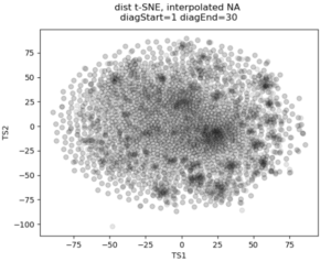
In the past I’ve attempted to visualize and cluster single-cell chromatin structure data. Pretty much any way I tried, on simulated and true experimental data, resulted the “cloud” – no real variation captured by the axes. In this t-SNE plot from simulated 3D structures collapsed to 2D maps, you can see some regions of higher density, but no true clusters emerging. The output layer of the autoencoder ideally contains much of the information in the original image, at a much reduced size. By clustering this output, we will hopefully capture more meaningful variation and better discrete grouping.


Groupings of similar folding in the 3D structure!

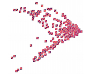
Here are the results of clustering the reduced dimensionality representations learned by the autoencoder. I’m using the PHATE method here, which seems especially applicable if chromatin is thought to have the ability to diffuse through a set of states. Each point is represented by the decoded output in this map. You can see images with similar structure, blocks that look like topologically associated domains, start to group together, indicating similarities in the input. There’s still much work to be done here, and I don’t think clear clusters would emerge even with perfect data – the space of 3D structures is just too continuous.

Denoising and inpainting

I am particularly surprised and impressed with the usage of deep learning for image superresolution and image inpainting. The results of some of the state of the art research are shocking – the network is able to increase the resolution of a blurred image almost to original quality, or find pixels that match a scene when the information is totally absent.

With these ideas in mind, I thought I could use a similar approach to reduce noise and “inpaint” missing data in simulated chromatin structures. These tasks also use an autoencoder/decoder architecture, but I don’t care about the size of the latent space representation so the model can be much larger. In experimental data obtained from high-powered fluorescence microscope, some points are outliers: they appear far away from the rest of the structure and indicate something went wrong with hybridization of fluorescence probes to chromatin or the spot fitting algorithm. Some points are entirely missed, when condensed to a 2D map these show up as entire rows and columns of missing data.
To train a model to solve these tasks, I artificially created noise or missing data in the simulated structures. Then the autoencoder/decoder was trained to predict the original, unperturbed distance matrix.

Here’s an example result. As you can see, the large scale features of the distance map are recovered, but the map remains noisy and undefined. Clearly the model is learning something, but it can’t perfectly predict the input distance map

Conclusions

By transferring a problem of 3D points to a problem of 2D distance matrices, I was able to use established deep learning techniques to work on single-cell chromatin structure data. Here I only showed simulated structures, because the experimental data is still unpublished! Using an autoencoder/decoder mode, we were able to better cluster distance maps into groups that represent shared structures in 3D. We were also able to achieve moderate denoising and inpainting with an autoencoder.

If I was going to continue this work further, there’s a few areas I would focus on:

  • Deep learning on 3D structures themselves. This has been used in protein structure prediction [ref]. You can also use a voxel representation, where each voxel can be occupied or unoccupied by a point. My friend Eli Draizen is working on a similar problem.
  • Can you train a model on simulated data, where you have effectively infinite sample size and can control properties like noise, and then apply it to real-world experimental data?
  • By working exclusively with 2D images we lose a lot of information about the input structure. For example the output distance maps don’t have to obey the triangle inequality. We could use a method like Multi-Dimensional Scaling to get a 3D structure from an outputted 2D distance map, then compute distances again, and use this in the loss function.

Overall, though this was an interesting project and a great way to learn about implementing a deep learning model in Keras!


k-mers are everywhere!

Many problems in bioinformatics involve working with short pieces of DNA sequence. We call these short words k-mers, where k is an integer usually less than 30 or so. A k-mer is essentially a substring of a larger sequence of DNA. If you’re  a biologist you may be wondering why people could be interested in anything other than 3-mers, the codons that encode amino acids. As it turns out, k-mers are at the center of many bioinformatics techniques and are the subject of intense algorithms research.

Some bioinformatics areas where k-mers play a central role:

  • Genome Assembly. Assemblers based on the overlap-consensus model (such as Celera) or De Bruijn Graphs (like Velvet) use k-mers to build the initial data structure for genome assembly. As overlaps between k-mers are found, the assembled sequence grows!
  • Sequence Alignment. The Basic Local Alignment Search Tool, or BLAST, is arguably the most well-known product of the bioinformatics field. BLAST can find DNA sequences conserved between organisms, uncover horizontal gene transfer and explain why we can’t make a vaccine for the common cold. And it all depends on the initial matching of short k-mers from the search sequence to the database.
  • Sequencing Quality Control. Overrepresentation of k-mers in a next gen sequencing library can be diagnostic for errors and duplications. The fastqc program computes the usage of 5-mers in sequencing reads as a form of quality control.
  • Alignment-Free sequence Analysis. My new favorite problem! Expect a post on this soon. Basically, the usage of short k-mers in a genome can be used to infer evolutionary relationships and examine horizontal gene transfer. Kind of like GC content but with more signal.
  • Codons and Repetitive Regions. Codons, the 3-letter sequences that encode for amino acids that build proteins, are essentially 3-mers with special biological function. 3-mers are also important in disease, such as the CAG repeats that cause Huntington’s disease.

K-mers are everywhere in bioinformatics. There is a lot of work into ways to efficiently (computational time and memory) count k-mers in large genomes. Really impressive and cool algorithms have been developed to solve the k-mer counting problem, some of which I’ll be talking about in a later post. It turns out these little words of DNA are important after all!