In my last post, I described how to simulate ensembles of structures representing the 3D conformation of chromatin inside the nucleus. Now, I’m going to describe some of my research to use deep learning methods, particularly an autoencoder/decoder, to do some interesting things with this data:
- Cluster structures from individual cells. The autoencoder should be able to learn a reduced-dimensionality representation of the data that will allow better clustering.
- Reduce noise in experimental data.
- Predict missing points in experimental data.
Something I learned early on rotating in the Kundaje lab at Stanford is that deep learning methods might seem domain specific at first. However, if you can translate your data and question into a problem that has already been studied by other researchers, you can benefit from their work and expertise. For example, if I want to use deep learning methods on 3D chromatin structure data, that will be difficult because few methods have been developed to work on point coordinates in 3D. However, the field of image processing has a wealth of deep learning research. A 3D structure can easily be represented by a 2D distance or contact map – essentially a grayscale image. By translating a 3D structure problem into a 2D image problem, we can use many of the methods and techniques already developed for image processing.
Autoencoders and decoders
The primary model I’m going to use is a convolutional autoencoder. I’m not going into depth about the model here, see this post for an excellent review. Conceptually, an autoencoder learns a reduced representation of the input by passing it through (several) layers of convolutional filters. The reverse operation, decoding, attempts to reconstruct the original information from the reduced representation. The loss function is some difference between the input and reconstructed data, and training iteratively optimizes the weights of the model to minimize the loss.

In this simple example, and autoencoder and decoder can be thought of as squishing the input image down to a compressed encoding, then reconstructing it to the original size (decoding). The reconstruction will not be perfect, but the difference between the input and output will be minimized in training. (Source)
Data processing
In this post I’m going to be using exclusively simulated 3D structures. Each structure starts as 64 ordered 3D points, an 64×3 matrix with x,y,z coordinates. Calculating the pairwise distance between all points gives a 64×64 distance matrix. The matrix is normalized to be in [0-1]. The matrix is also symmetric and has a diagonal of zero by definition. I used ten thousand structures simulated with the molecular dynamics pipeline, with an attempt to pick independent draws from the MD simulation. The data was split 80/20 between training and
Model architecture
For the clustering autoencoder, the goal is to reduce dimensionality as much as possible while still retaining good input information. We will accept modest loss for a significant reduction in dimensionality. I used 4 convolutional layers with 2×2 max pooling between layers. The final encoding layer was a dense layer. The decoder is essentially the inverse, with upscaling layers instead of max pooling. I implemented this model in python using Keras with the Theano backend.
Dealing with distance map properties
The 2D distance maps I’m working with are symmetric and have a diagonal of zero. First, I tried to learn these properties through a custom regression loss function, minimizing the distance between a point i,j and its pair j,i for example. This proved to be too cumbersome, so I simply freed the model from learning these properties by using custom layers. Details of the implementation are below, because they took me a while to figure out! One custom layer sets the diagonal to zero at the end of the decoding step, the other averages the upper and lower triangle of the matrix to enforce symmetry.
Clustering single-cell chromatin structure data
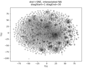
In the past I’ve attempted to visualize and cluster single-cell chromatin structure data. Pretty much any way I tried, on simulated and true experimental data, resulted the “cloud” – no real variation captured by the axes. In this t-SNE plot from simulated 3D structures collapsed to 2D maps, you can see some regions of higher density, but no true clusters emerging. The output layer of the autoencoder ideally contains much of the information in the original image, at a much reduced size. By clustering this output, we will hopefully capture more meaningful variation and better discrete grouping.
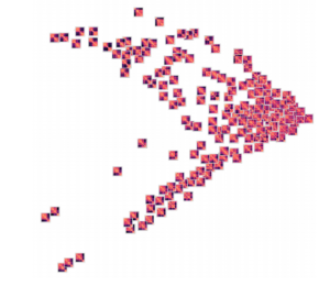
Here are the results of clustering the reduced dimensionality representations learned by the autoencoder. I’m using the PHATE method here, which seems especially applicable if chromatin is thought to have the ability to diffuse through a set of states. Each point is represented by the decoded output in this map. You can see images with similar structure, blocks that look like topologically associated domains, start to group together, indicating similarities in the input. There’s still much work to be done here, and I don’t think clear clusters would emerge even with perfect data – the space of 3D structures is just too continuous.
Denoising and inpainting
I am particularly surprised and impressed with the usage of deep learning for image superresolution and image inpainting. The results of some of the state of the art research are shocking – the network is able to increase the resolution of a blurred image almost to original quality, or find pixels that match a scene when the information is totally absent.
With these ideas in mind, I thought I could use a similar approach to reduce noise and “inpaint” missing data in simulated chromatin structures. These tasks also use an autoencoder/decoder architecture, but I don’t care about the size of the latent space representation so the model can be much larger. In experimental data obtained from high-powered fluorescence microscope, some points are outliers: they appear far away from the rest of the structure and indicate something went wrong with hybridization of fluorescence probes to chromatin or the spot fitting algorithm. Some points are entirely missed, when condensed to a 2D map these show up as entire rows and columns of missing data.
To train a model to solve these tasks, I artificially created noise or missing data in the simulated structures. Then the autoencoder/decoder was trained to predict the original, unperturbed distance matrix.
Here’s an example result. As you can see, the large scale features of the distance map are recovered, but the map remains noisy and undefined. Clearly the model is learning something, but it can’t perfectly predict the input distance map
Conclusions
By transferring a problem of 3D points to a problem of 2D distance matrices, I was able to use established deep learning techniques to work on single-cell chromatin structure data. Here I only showed simulated structures, because the experimental data is still unpublished! Using an autoencoder/decoder mode, we were able to better cluster distance maps into groups that represent shared structures in 3D. We were also able to achieve moderate denoising and inpainting with an autoencoder.
If I was going to continue this work further, there’s a few areas I would focus on:
- Deep learning on 3D structures themselves. This has been used in protein structure prediction [ref]. You can also use a voxel representation, where each voxel can be occupied or unoccupied by a point. My friend Eli Draizen is working on a similar problem.
- Can you train a model on simulated data, where you have effectively infinite sample size and can control properties like noise, and then apply it to real-world experimental data?
- By working exclusively with 2D images we lose a lot of information about the input structure. For example the output distance maps don’t have to obey the triangle inequality. We could use a method like Multi-Dimensional Scaling to get a 3D structure from an outputted 2D distance map, then compute distances again, and use this in the loss function.
Overall, though this was an interesting project and a great way to learn about implementing a deep learning model in Keras!


