Much of the current evidence for the loop extrusion hypothesis comes from molecular dynamics simulations. In these simulations, DNA is modeled as a polymer, loop extruding factors with certain parameters are added into the mix, and the polymer is allowed to move around as if it were in a solvent. By running the simulation for a long time and saving conformations of the polymer at defined intervals, you can gather an ensemble of structures that represent how chromatin might be organized in a population of cells. Note that molecular dynamics is much different than MCMC approaches to simulating chromatin structure – here we’re actually simulating how a chromatin might behave due to physical and chemical properties.

In this post, I’m going to show you how you can run these molecular dynamics simulations for yourself. The simulations rely on the OpenMM molecular simulation package, the Mirnylab implementation of openmm-polymer and my own scripts and modification of the mirnylab code.

Ingredients

• Install the required packages. See the links above for required code repositories. Note that it can be quite difficult to get openmm-polymer configured properly, so good luck…
• Simulation is much quicker using a GPU
• Pick your favorite chromatin region to simulate. In this example, we’re going to use a small region on chromosome 21.
• Define CTCF sites, including orientation and strength. These will be used as blocking elements in the simulation. The standard is to take CTCF binding ChIP-Seq data for your cell type of interest, overlap the peaks with another track too add confidence and determine orientation (such as CTCF motifs in the genetic code or RAD21 binding data).
• Define other parameters for the simulation, such as the time step and number of blocks to save. These can be found in the help text for the simulation script.

Check your parameters

Before running a time consuming 3D polymer simulation, you can run simple test to see how the extruding factors are behaving in the simulation. This 2D map gives the probability of an extruder binding two sites along the linear genome, and is a good prediction for how the mean 3D structure will look. Briefly, there’s a logistic scaling function that transforms an arbitrary ChIP-Seq peak strength into a 0.0-1.0 interval. The scaled strength of the each site defines the probability that a LEF can slip past the site without stalling. Even though CTCF might form an impermiable boundary in reality, modeling this with a probability makes sense because we’re generating an ensemble of structures. You might need to tune the parameters of the function to get peak strengths to make sense for your ChIP-Seq data.

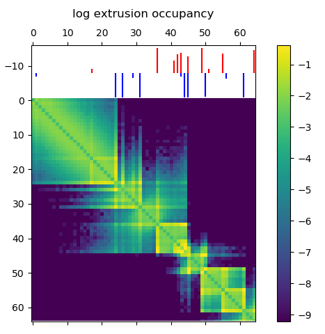
Loop extruder occupancy matrix. This gives the log transformed probability of a LEF binding two locations along the genome. CTCF sites for the example region of interest are shown above, with the color indicating directionality and height indicating strength. Notice how we already start to see domain-like structures!

Running the simulation

With all the above ingredients and parameters configured, it’s time to actually run the simulation. Here we will run for a short number of time steps, but you should actually let the simulation run for much longer to gather thousands of independent draws from the distribution of structures.

Using the code available at my github, run the loop_extrusion_simulation.py script. Here is an example using the data available in the repository

cd openmm-dna
python src/loop_extrusion_simulation.py -i data/example_ctcf_sites.txt -o ~/loop_extrusion_test --time_step 5000  --skip_start 100 --save_blocks 1000

Some explanation of the parameters: time_step defines how many steps of simulation are done between saving structures, skip_start makes the script skip outputting the first 100 structures to get away from the initial conformation, save_blocks means we will save 1000 structures total. There are many other arguments to the script, check the help text for more. In particular, the –cpu_simulation flag can be used if you don’t have a GPU.

If everything is configured correctly, you’ll see output with statistics on the properties of each block.

potential energy is 3.209405
bl=1 pos[1]=[10.9 14.2 5.8] dr=1.46 t=8.0ps kin=2.39 pot=2.24 Rg=9.084 SPS=235
Number of exceptions: 3899
adding force HarmonicBondForce 0
adding force AngleForce 1
Add exclusions for Nonbonded force
Using periodic boundary conditions!!!!
adding force Nonbonded 2
Positions...
loaded!
potential energy is 2.354693
bl=2 pos[1]=[11.4 14.1 6.0] dr=1.21 t=8.0ps kin=1.78 pot=2.09 Rg=9.278 SPS=333
...

Processing simulated structures

After simulation, I process the raw structures by trimming the ends (by the same amount of the –extend argument) and binning the points by taking the 3D centroid to reduce the resolution. As I’m trying to match experimental data with this simulation, I reduce the resolution to the same as the experimental data. Then I save the ensemble in a numpy array, which is much quicker to load for subsequent analysis. There’s a script to do this:

python src/process_simulated_structures.py -i ~/loop_extrusion_test -o ~/loop_extrusion_test/processed

Analysis of results

There are a few ways you can analyze the results after the simulation has finished. The obvious first step is to create an average contact map from the ensemble of structures. This plot is the most comparable to a Hi-C dataset.

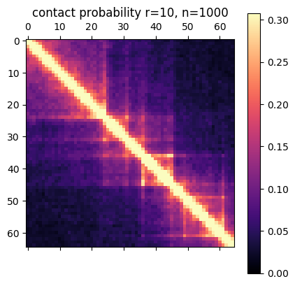
Simulation contact probability at radius of 10. 1000 structures went into this plot.

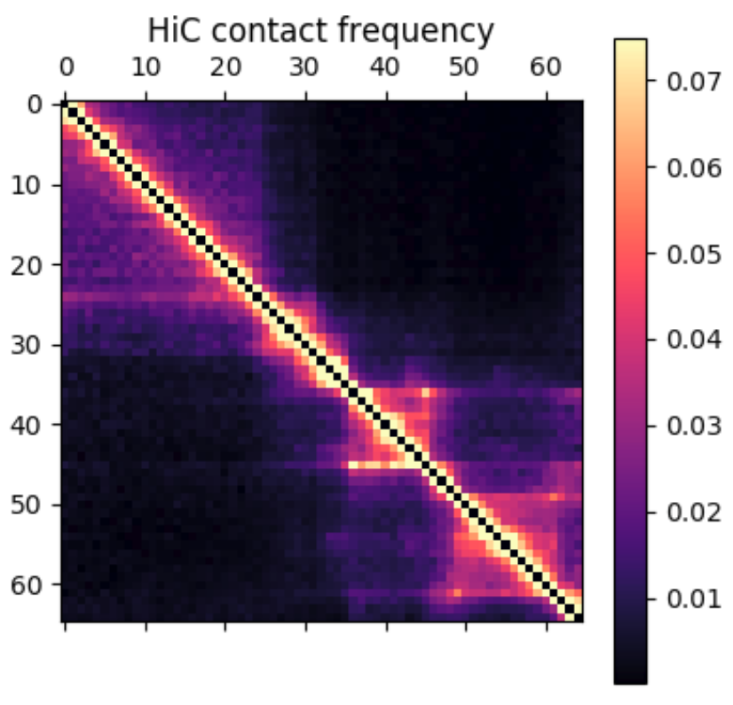
Hi-C contact frequency for the same region in K562 cells. A great qualitative match, inluding domains and peaks!

Another common way to look at chromatin structure data is plotting contact probability as a function of genomic distance. This function is expected to decrease linearly on a log-log plot, with the slope giving evidence for mechanism for packing the underlying structures. You can look at the radius of the structures, how they cluster, and many other metrics. More on this to come later!