Reducing RNA-seq batch effects by re-aligning TCGA and GTEx

At Pattern, we want to be able to compare RNA-seq data between several public sources and our growing internal datasets. We care a lot about the differential expression of certain genes, but batch effects can completely overwhelm any signal of genes overexpressed in cancer, genes changing between cancer subtypes, and similar comparisons.

A few publications [1,2] suggest that processing raw, read-level data from different public sources with a consistent bioinformatics pipeline can reduce the batch effects in RNA-seq. That makes sense — I can imagine the batch effect is the sum of effects from cohort selection, sample collection, sample processing, library preparation, sequencing, and bioinformatics methods. Eliminating the contribution of bioinformatics to this equation can surely reduce the overall batch effect, but is it enough to be noticeable? Is it worth the extra computational effort?

Several months ago, I began the journey to consistently process all the samples from The Cancer Genome Atlas (TCGA, the largest public collection of RNA-seq data from different cancers), the Genotype Expression project (GTEx, the largest collection of RNA-seq data from many tissues of healthy individuals), and our internal collection of several hundred tumor and normal RNA-seq samples. The total was over 30,000 samples and 200TB of raw data. I used the nf-core/rnaseq pipeline, since that’s what I already ran for internal data. The challenges I encountered along the way are the subject of this post.

If you only make it this far, I think it is worth it to re-process RNA-seq data whenever raw reads are available. The reduction in batch effects, as measured by decrease in distance between centroids in PCA-space of different datasets, was larger than I expected. I’ve started always going back to raw reads for public RNA-seq data when they are available.

Challenge 1: Getting access to the raw data.
Raw, read-level data for TCGA and GTEx is only available behind an application to NIH because it has information on germline genetic variants. Yes, you can get access to controlled data in industry. This is not clear by looking at the NIH dbGaP documentation, but all it takes is one person at the company to register in eRA Commons as the Signing Officer, and you to register as the PI. Then, just complete the application for each dataset, correct the mistakes you will inevitably make, and wait a few weeks.

Challenge 2: Where are you going to run all these alignments?
I thought about running these 30k samples on AWS, but even with spot instances, the total cost would have been $20k-$30k. Instead, I chose to buy a few servers for about the same price. Now that the project is over, I still have the hardware, and my cloud bill stayed sane. The workhorse of the project was a dual AMD EPYC 9654 machine (192 cores, 384 threads) with 1.5TB of RAM and 30T of local NVMe storage. It’s networked at 100Gb/s to a storage server with 100TB of NVMe. This is a subset of the hardware build-out I did when we moved to our new office, which should be the topic of a separate post.

Challenge 3: Downloading 200TB of raw fastq files.
Downloading TCGA controlled access data with the gdc-client tool works well. GTEx on the other hand… is another story. Despite the fact that our taxpayer dollars paid for every aspect of the GTEx project, the GTEx raw data is only available in Google Cloud Storage. I have to pay Google for permission to use the sequencing data that I already paid to collect! It would cost something like $12k to download the entirety of GTEx so I could process it on my new servers, which were sitting idle after enthusiastically consuming all of the TCGA data with no sign of slowing down. If only there was a better way…
If you read the Google Cloud Storage docs closely, you’ll notice something in the fine print. Egress from Google Cloud to Google Drive is FREE. And downloading from Google Drive is never charged. We already pay for 10s of TB of space in Drive through our Google Workspace subscription. The path emerged:
Google Cloud Storage -> Google Cloud VM -> Google Drive -> Local servers. Zero egress charges.
The only issues are a 750GB upload limit to Google Drive per user per day, but service accounts count as a user for the purposes of this limit. I had a path forward! Finally, both TCGA and GTEx provide aligned BAM files, but the raw reads can be extracted with samtools fastq. GTEx reads required sorting before alignment.

Challenge 4: Actually running 30k samples through nf-core/rnaseq
I had to work in batches due to the large amount of temporary files that are generated during the nf-core/rnaseq pipeline. Processing everything at once would have generated 2PB in temporary files and results! I set up a script to launch batches of 500 samples at a time, upload the results I cared about to AWS, and delete everything else when the batch was complete.
I did some minor tuning to the pipeline, including disabling tools I didn’t need and changing the job resource requirements to better match my hardware. It took about 45 days of continuous runtime to process all the samples.

Results

I looked at groups of samples from matched organs from the different datasets to quantify the batch effects before and after re-processing. For GTEx, nTPM (normalized transcripts per million) normalization was done across the entire collection. For TCGA, normalization was done per-project. PCA was calculated for all samples from a matched organ. The centroid of the points from each dataset was estimated in 2D or Nd space, and the euclidean distance between centroids was calculated. A distance was also calculated using only non-tumor samples in TCGA, which were expected to be closer in PC-space to the GTEx samples. All of these results are before running any batch correction algorithm, like COMBAT.

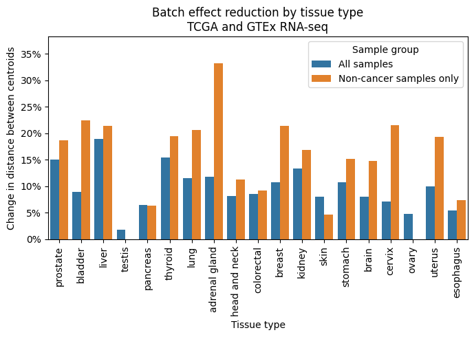
In every matched organ, re-processing TCGA and GTEx RNA-seq samples with a consistent bioinformatics pipeline reduced the batch effects. The reduction was almost always larger when considering only non-tumor samples.

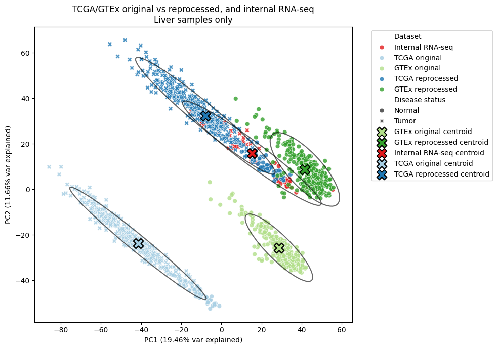
In the liver, where we have the most internal RNA-seq data, all three data sources were much closer in PC-space after re-processing. I’m particularly happy about this result, as it means our internally-generated data can be compared with these external sources more reliably.

References

  1. Arora, S., Pattwell, S. S., Holland, E. C. & Bolouri, H. Variability in estimated gene expression among commonly used RNA-seq pipelines. Sci Rep10, 2734 (2020).
  2. Wang, Q. et al. Unifying cancer and normal RNA sequencing data from different sources. Sci Data5, 180061 (2018).

s3stasher simplifies using AWS S3 in python

Working with cloud files in python is a necessary pain at any biotech organization. While packages like pandas transparently handle S3 URIs, I still found myself writing the same boto3 code to manage files far too often. Nextflow solves this for workflows, but there aren’t any packages that I’m aware of that make managing S3 files easier for script and notebook use cases.

I developed s3stasher to make working with files in AWS S3 as easy if they were local files. The key principles are:

  • S3 objects should be referred to as full URIs at all times. It shouldn’t be necessary to split a URI into bucket and key strings.
  • Any method that reads or writes a file should transparently work on S3 URIs or local files.
  • S3 objects should be cached locally and only re-downloaded when the source object has changed.
  • Reading S3 objects should work identically while offline, assuming the user has the file cached.

Using s3stasher, you simply have to wrap any file reading or writing in a with statement, and all the file operations will happen behind the scenes.

from s3stasher import S3

# Download, cache, and read an S3 object
with S3.s3open("s3://my-bucket/my_data.csv") as f:
    my_df = pd.read_csv(f)

# Two layers of context manager are needed for traditional open operations
with S3.s3open("s3://my-bucket/unstructured.txt") as s3f:
    with open(s3f) as f:
        lines = f.readlines()

# Write a file back to s3. By default, it will be saved in the cache dir 
# to avoid an unnecessary download in the future
with S3.s3write("s3://my-bucket/my_data_new.csv") as f:
    my_df.to_csv(f)

# Other convenience functions are provided
## List objects under a prefix
uri_list = S3.s3list("s3://my-bucket/prefix/")
## Check for existance of an object
uri_exists = S3.s3exists("s3://my-bucket/unknown_file.txt")
## copy, move, remove an S3 object
S3.s3cp("s3://my-bucket/my_file_1.txt", "s3://my-bucket/my_file_2.txt")
S3.s3mv("s3://my-bucket/my_file_2.txt", "s3://my-bucket/my_file_3.txt")
S3.s3rm("s3://my-bucket/my_file_3.txt")

By default, s3stasher uses your already set up AWS credentials, and caches files to ~/.s3_cache. All of these options can be changed with a config file or environment variables.

You can install s3stasher with a quick pip install s3stasher.
Pypi: https://pypi.org/project/s3stasher/
GitHub: https://github.com/bsiranosian/s3stasher

Feedback and PRs welcome!

Does AMD 3D V-Cache help in bioinformatics?

Introduction

In our new office at Pattern, I have 42U of server rack space to play with, so I want to get an AMD EPYC server for some long-running bioinformatics tasks. EPYC Genoa looks like the sweet spot for price to performance, but which of the 24 SKUs is the best for typical bioinformatics workloads? Obviously, more cores and more frequency is more better, but are there additional factors to consider?

Specifically, I’m interested in comparing the 9654 and 9684X CPUs. Both are 96-core, 192 thread monsters that can boost up to 3.7 GHz, but the 9684X has over a gigabyte of L3 cache, three times that of the 9654. That’s AMD 3D V-Cache, which became famous through it’s use in gaming desktop CPUs and has now made its way to the server market. 3D V-Cache is also supposed to help certain productivity workloads, but there’s not many benchmarks that cover bioinformatics specifically. The only mention I could find was this post on Mark Ziemann’s blog.

AMD 3D V-Cache diagram

The cache is stacked on top of the processor … in 3D!

In this post, I benchmark a few common bioinformatics tools with the AMD 7950X3D processor, which has both 3D V-Cache and normal cores. In the end, I’m surprised to find a little to no increase in performance when running on the 3D V-Cache cores, at least for the algorithms I tested.

Methods

  • Processor: AMD Ryzen 9 7950X3D: 16-core / 32-thread. 2 × 8‑core Core Complex Dies (CCDs). One CCD has 3D V-Cache. 128 MB L3 cache total, split 96/32 across the different CCDs.
  • BIOS setup: For the V-Cache test, I disabled the non‑V-Cache CCD in BIOS. The reverse was done for the non V-Cache test.
  • Operating system: Ubuntu 22.04.
  • Other hardware: 2TB M.2 SSD, 96GB RAM. Memory overclocking and Precision Boost Overdrive (PBO) were disabled for this test.
  • The V-Cache CCD boosts up to ~4.8 GHz under load, but the non V-Cache CCD can reach ~5.8GHz. To control for frequency, I ran a third test locking the non‑V-Cache CCD at 4.8 GHz via the cpupower command.
  • Bioinformatics tools: We do a lot of short and long-read alignment, so I used minimap2, STAR, and a full run of the nf-core/RNAseq pipeline. All with real-world data from one sample.
  •  Measurement: Wall time for the completion of the single command or entire pipeline. Average of 3 replicates reported for each test. The results of each test were surprisingly tight, within a few seconds. The same datasets and command were used for each test. Non-essential background processes as possible were closed during the test.

Results

Processor sectionSTAR (s)minimap2 (s) nf-core/RNAseq (m)
V-Cache CCD 4.8 GHz36849360.1
Non V-Cache CCD 5.8 GHz
35442754.2
Non V-Cache CCD 4.8 GHz38446963.2
V-Cache improvement compared to 5.8 GHz-3.8%-15.5%-10.9%
V-Cache improvement compared to 4.8 GHz4.2%-5.1%4.9%

These results were quite interesting. 3D V-Cache offers a modest improvement compared to a frequency-matched processor, but only for certain tools and workflows. When the non V-Cache CCD was allowed to use the full 5.8GHz, it was always the winner.

Conclusions

For alignment-based bioinformatics tasks, a processor with 3D V-Cache may gain a task-dependent and small improvement in runtime. These improvements were completely negated by a higher-frequency processor. This is nowhere near the halving of runtime seen with computational fluid dynamics and other workloads.

Buying the more expensive and higher powered EPYC 9684X likely isn’t worth it for my use case. I need to learn more about how these algorithms take advantage of different CPU cache levels in order to attempt to explain these results. Additional investigation with AMD μprof might be helpful.

These results significantly more modest than what was reported at Genome Spot, although that post looked at Intel processors.

Limitations

These results could differ for other bioinformatics tasks, like variant calling. Additionally, I attempted to simulate the performance difference of two separate server processors by using different CCDs on my desktop processor. This method could give different results than separate server CPUs.

Cross-account AWS FSx for Lustre and S3 data repository associations

FSx for Lustre and S3 are two complementary methods of storing data in Amazon Web Services (AWS). FSx offers an extremely performant, reliable, true filesystem, but it’s expensive and not accessible via the web or other APIs. S3 offers cheaper object storage that’s accessible from any device connected to the internet, but methods to access objects in S3 as files are limited.

AWS does have a great feature where you can set up a data repository association between a FSx for Lustre filesystem and n S3 bucket. This lets you sync the contents of the filesystem and the bucket, either in one direction or bidirectionally. This is helpful for users who want to access data from a traditional file path on a filesystem, but the data lives in S3. It’s also good if users also want to output results onto the filesystem, but other teams want to access the results from S3.

AWS supports linking FSx and S3 resources in different accounts, and even in different regions (FSx to S3 export only). However, nowhere in the documentation does AWS cover how to configure permissions to enable cross-account data repository associations.

At Deep Origin, we just set this up to let one of our customers access data in a S3 bucket as files in a ComputeBench. I wanted to share a simplified version of bucket polices in case anyone was searching the internet for the same answer!

To access a bucket via the “import” read-only data repository association, add this policy to the source bucket. Change YOUR_BUCKET to the id of the source bucket, and ACCOUNT_WITH_FSx:user/USER to the IAM identifier of the account owning the FSx volume. You can then set up the data repository association from the account owning the FSx volume as you normally would.

<p>{ "Version": "2012-10-17", "Statement": [ { "Effect": "Allow", "Action": [ "s3:Get*", "s3:List*", "s3:PutBucketNotification" ], "Resource": [ "arn:aws:s3:::YOUR_BUCKET/*", "arn:aws:s3:::YOUR_BUCKET" ], "Principal": { "AWS": "arn:aws:iam::ACCOUNT_WITH_FSx:user/USER" } } ] }</p>


For a bucket policy that also allows export of data from FSx to S3, add a few write permissions:

<p>{ "Version": "2012-10-17", "Statement": [ { "Effect": "Allow", "Action": [ "s3:Get*", "s3:List*", "s3:PutBucketNotification", "s3:AbortMultipartUpload", "s3:DeleteObject", "s3:PutObject", ], "Resource": [ "arn:aws:s3:::YOUR_BUCKET/*", "arn:aws:s3:::YOUR_BUCKET" ], "Principal": { "AWS": "arn:aws:iam::ACCOUNT_WITH_FSx:user/USER" } } ] }</p>

Introducing the ComputeBench: the cloud development environment for bioinformatics

The following is a cross-post from the Deep Origin blog.

Today, I’m proud to announce the beta release of Deep Origin’s first product: the ComputeBench. The ComputeBench is a cloud-based environment for interactive analysis in computational biology and bioinformatics. It’s designed from the ground up for computational scientists – providing you the compute and storage resources you need, the software packages you expect, and tools for seamless collaboration with your team, all in a secure, backed-up and scalable platform.

We’re building Deep Origin for teams of computational scientists to work in a collaborative, cloud-based environment without worrying about DevOps and IT. In short, our mission is to let scientists focus on science. What we’re releasing today is the first stop in that longer-term vision. Read on to learn more about ComputeBenches, or check out the product page, pricing, and request access.

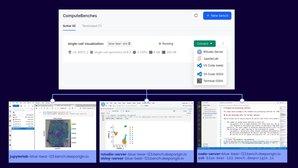
An overview of the ComputeBench.

After starting a ComputeBench, it’s one click to drop into the development environment you’re most comfortable with. Computational power, storage, and hundreds of packages are available at your fingertips!

Two trends in biological discovery highlight the importance of developing better tooling for computational biology:

  • Biological discoveries are increasingly driven by massive amounts of heterogeneous data. Look no further than the move to single-cell, spatial, long read, or multi-omic profiling, or the promises of the newest instrument vendors.
  • Biological discoveries are increasingly collaborative. In both academia and industry, science doesn’t happen in a vacuum, especially when an analysis spans different modalities and areas of expertise.

Meanwhile, tools for collaborative computational biology at scale are lacking, and scientists frequently waste hours or days solving problems that we are all too familiar with. How long have you spent troubleshooting a package installation, setting up the right infrastructure and permissions to share data with a collaborator, or reproducing an analysis from a publication? How many teams have built undifferentiated cloud infrastructure just to get to the point that they can start to do their job?

We built the ComputeBench for these scientists. We want to give every scientist superpowers to scale their analysis, without the boring stuff getting in the way. A ComputeBench has the following key features:

  • Scalable hardware: from 2-192 vCPU, 4-1536 GB of RAM, up to 16 TB of local persistent storage, and NVIDIA GPUs if you need them.
  • Software blueprints: collections of hundreds of pre-installed, validated, and versioned tools for different scientific domains. Use the tools in the blueprints, or use them as a jumping off point to customize and create your own environment. Examples of our blueprints include metagenomics, RNA sequencing, and single-cell sequencing.
  • Interact the way you want: Each blueprint provides a number of user-friendly web-based applications, like JupyterLab, RStudio, VS Code server, R Shiny, or CELLxGENE. You can also connect over SSH, and you have root access to modify your bench as you see fit.
  • Storage volumes: performant, scalable storage that can be accessed by all of your ComputeBenches to share data among your team.
  • Credential and secret management: Store your secrets and preferences, and automatically load them in every ComputeBench that you create. Share team-level variables and secrets, as well.
  • Usage and cost controls. Automatically stop idle ComputeBenches, and view transparent, up-front pricing before you create any resources.
  • Invoices for humans. Deep Origin customers receive invoices in terms that are easy to understand and traceable to a particular user or ComputeBench.

ComputeBenches provide the best experience for interactive analysis in computational biology – and we bet you’ll feel the same way. To get started, we’re offering new users $500 in credits to try working on the Deep Origin platform. Since much of the benefit of working on our platform comes when you are working with your team members, we’ll add $500 for each regular user you bring on to your organization, as well.

Claim your $500 in credits here.

Finally, we’re always looking for ways to improve the platform. Next on our roadmap are features allowing users to submit their own software blueprints for use within their organization, and tools to manage data in buckets, both hosted by Deep Origin and elsewhere. If you have feature requests, suggestions of packages to add to a blueprint, or other feedback, please let us know.

Accelerated computing is the future of genomics

“We’re out of storage, and we’re out of compute.” I’ll never forget the 2016 Broad Institute Cancer Program meeting where Eric Banks, senior director of the Data Sciences Platform, showed the audience how much genomic data the Broad was generating. The exponential curve was plotted against the current capacity of the on-premises compute cluster –  the time until intersection of the curves could be measured in months. In fact, we were generating data even faster than we could add new storage drives. This meeting sparked the Broad’s move to the cloud for the majority of data storage and compute.

While moving to the cloud may have been the simple answer seven years ago, it’s not a catch-all solution today. Genome sequencing costs have dropped precipitously, and newer high-content assays like single-cell sequencing and spatial transcriptomics are being developed every day. Storing and processing all these data requires a massive amount of resources, and a cloud bill to match (even if you’re trying to do the analysis on the cheap). We need new, more efficient ways to process, store and transfer genomic data. Enter accelerated computing.

Accelerated computing, the use of special-purpose hardware for specific computational tasks, can help solve many of the problems facing genomics today. Using Graphical Processing Units (GPUs) and similar hardware, these custom-developed algorithms can reduce the time needed to run an analysis by a factor of 10 to 100. This great reduction in compute time has paved the way for more efficient data processing and real-time analysis in clinical genomics.

In this series, I’ll cover three topics related to accelerated computing in genomics:

  • An overview of the basics of accelerated computing, the popular tools, and the companies developing them (this post).
  • Practical considerations. How can you use these tools today? (coming soon)
  • Algorithmic details. How do accelerated tools work to drastically decrease the runtime of common tasks? What problems in genomics are amenable to acceleration? (a future post)

Accelerated computing is a general term describing the use of specialized hardware to speed up a certain computation. Commonly used hardware in the genomics space includes:

  • Graphical Processing Units (GPUs)
  • Field Programmable Gate Arrays (FPGAs)
  • Application-specific integrated circuits (ASICs)
  • Tensor Processing Units (TPUs)

While Central Processing Units (CPUs) excel at general-purpose tasks, they lack the ability to run many computations in parallel. GPUs are the opposite. While they were originally developed for video game rendering, GPUs excel at parallel computations. They can have thousands of processor cores, each capable of running a calculation in parallel. Accelerated computing takes advantage of each hardware type for the tasks it is best at. Control functionality and single-threaded work is left to the CPU, and parallelizable computations are done on the GPU. NVIDIA Clara Parabricks leads the way in GPU-accelerated genomics.

FPGAs allow for the hardware to be reconfigured on the fly to run a specific algorithm. They are used in the Illumina DRAGEN tools I’ll cover later. ASICs are less common. They have a fixed configuration and perform a limited set of functions, so they’re best used in very specific settings, like controlling the pores on an Oxford Nanopore MinION. TPUs are used in training ML models to interpret genomic data, but not in the processing of the data directly.

While GPU-based training of deep learning models is standard and supported by key libraries in the ecosystem, in traditional genomics fashion, the field is 5-10 years behind other industries. We are starting to see GPU-based genomics tools being released, but they’re closed source and still gaining traction. By contrast, PyTorch, a popular open source machine learning framework, was released in 2016! My prediction is that accelerated tools will become standard in genomics as well, but we need a lot of work to get there.

How can I use hardware acceleration in genomics today?

Your best bet is to use one of these developed toolkits. If you don’t have access to a machine with GPUs or FPGAs, they can be rented from AWS or GCP for a low hourly fee.

NVIDIA Clara Parabricks: GPU-accelerated alignment, variant calling, and RNA-seq

NVIDIA’s entry into GPU-accelerated genomics is the result of the 2019 acquisition of the software startup Parabricks. NVIDIA first released the software as closed access, but with the version 4.0 release in 2022, anyone can download the docker container and run the software. Parabricks runs on most modern NVIDIA GPUs and accelerates alignment of DNA and RNA-seq data, variant calling, and other time-intensive processes by up to 80x (using a multi-GPU machine). Parabricks was designed as a drop-in replacement for common tools like GATK, and is guaranteed to produce an identical output as certain GATK versions. Running the software is simple, all you have to do is pull the docker container at nvcr.io/nvidia/clara/clara-parabricks:4.0.0-1 and run one of the command line tools.

The strengths of Parabricks lie in its ease of use, wide applicability, and cost effectiveness. GPUs are everywhere: on the cloud, in gaming PCs, and in servers used for ML/AI training. The docker container is available for anyone to try for free, without a license or multiple sales calls. Parabricks also attempts to automate some processes that may have been spread across multiple tools in the past: alignments are always  coordinate-sorted, for example.

The weaknesses of Parabricks come down to the limited functionality and lack of integration, at least compared to DRAGEN. Parabricks doesn’t have the advanced functionality of DRAGEN for tasks like single-cell sequencing and star-allele calling for pharmacogenomics. And you obviously can’t buy an Illumina sequencer with a competitor’s hardware and software in it!

Illumina DRAGEN: FPGA-accelerated Bio-IT platform

Illumina recognized the challenges in storage and processing of genomic data early, and acquired Edico Genome and the DRAGEN Bio-IT platform in 2018 to architect a solution. DRAGEN uses FPGAs to speed up generation of FASTQ files, alignment, variant calling, and many other processes. In addition to a standard GATK implementation, DRAGEN designed their own variant calling algorithms which have won two out of three of the Precision FDA Truth Challenge V2 Illumina categories. DRAGEN also provides new algorithms for accelerated single-cell genomics, star-allele calling, and other processes.

The strengths of DRAGEN lie in the tight integration with Illumina products. You can buy an Illumina sequencer with a DRAGEN server built in, so that everything up to variant calling can be completed on the sequencer. This means the large raw data files never have to be transferred to the cloud or elsewhere, saving on storage costs (as long as you don’t need the raw data for backup or compliance purposes). The accuracy, speed, and continued improvement of the algorithms are another key advantage.

The weaknesses of DRAGEN come with the costs of using the software. Since Illumina doesn’t benefit from the purchase of FPGAs, they charge a LOT for the DRAGEN license. In fact, the license cost is 80% of the total cost when running DRAGEN on the cloud! This deters researchers in academia and lower-resourced companies from using DRAGEN, and may push them to a free alternative instead.

Nanopore and PacBio sequencers: accelerated computing right under the hood

Oxford Nanopore uses hardware acceleration at multiple places in their long-read sequencers. Pores on the flowcells are controlled by ASICs, and the more advanced multi-flowcell workstations use GPUs to accelerate data analysis. The Nanopore Promethion comes with 4 NVIDIA A100 GPUs, for example. PacBio’s new Revio sequencer has a similar arrangement, with on-board GPUs to speed up the processing of raw data. While Nanopore and PacBio sequencers both take advantage of hardware acceleration, there’s much less direct interaction with the algorithms, compared to the user-facing toolkits above.

Where’s the PyTorch of genomics?

All of the accelerated genomics toolkits I’ve talked about today are being developed closed-source by publicly traded companies. That’s great for efficient development of high-performance code, but it shuts out the community of developers in academia or low-resource industries that might use and contribute to your code. NVIDIA had GenomeWorks, but that hasn’t seen a commit in a year and a half. Some other groups are repurposing GPU-accelerated Python libraries for single-cell analysis.

If you’re working on an open-source GPU genomics toolkit, I’d love to hear about it.

One final thought: the story of how GPUs transitioned from gaming devices to general-purpose compute accelerators is both fascinating and entertaining. It all started with a quantum chemistry professor at Stanford buying NVIDIA gaming cards in 2006 and hacking them to do the computation he needed. Acquired has a great podcast on the topic.

Bioinformatics in the cloud, on a budget

Let’s say you’re a biotech or academic lab that needs to do bioinformatics or computational biology at a reasonably large scale. You have a tight budget and you want to be as cost effective as possible. You also don’t want to build and maintain your own hardware, because you recognize the hidden costs baked into the time, effort, and security of doing so. Luckily, the last few years have seen a proliferation of “alternative” cloud providers. These providers can compute with AWS, GCP and Azure by doing few things really well at greatly reduced prices. My main argument in this post is that by mixing services from different cloud providers, budget and cloud can mix, despite the prevailing pessimistic opinions. 

To be upfront, I believe working with one of the larger public cloud providers will make your life easier and allow you to deliver results faster, with less engineering expertise. AWS has services that cover everything a biotech needs to process data in the cloud, and the integration between these services is seamless and efficient. But we’re not going for easy here, right? We’re going for cheap. And cheap means cutting some corners and making things more difficult in the name of saving your valuable dollars.

What’s the problem with the big public cloud providers? AWS allows a team to build any product imaginable, and scale in infinitely. Need to build a Netflix competitor that can deliver video with low latency and maximum uptime to every corner of the world? AWS will let you do that (and bill you appropriately). With this plethora of features comes many hidden costs. It can seem like AWS intentionally makes their billing practices opaque, allowing you to rack up massive bills by leaving a service running or enabling features you don’t need. In the future, I’ll do a separate post on keeping AWS costs manageable. For now, just know that you have to be careful or you can be burned – I personally know several individuals that have made costly mistakes here. Even when just looking at raw compute, AWS is priced at a large premium compared to competitors on the market. You pay for the performance, uptime, reliability, interoperability, and support.

The minimum viable bioinformatics cloud

With that out of the way, it’s time to design our bioinformatics cloud! The minimum capabilities of a system supporting a bioinformatics team include: 

    1. Interactive compute for experimentation, prototyping workflows, programming in Jupyter and RStudio and generating figures. GPUs may be needed for training machine learning models. 
    2. Cloud storage that’s accessible to all team members and other services. Ideally this system supports cheap cold storage for infrequently accessed and backup data.
    3. Container registries. Batch workflows need to access a high-bandwidth container registry for custom private and public containers. 
    4. Scalable batch compute that can be managed by a workflow manager. A team should be able to easily 10-1000X their compute with a single command line argument or config change.
    5. GPUs, databases, and other add-ons, depending on the work the team is doing. 

Where can we cut corners?

Some of the features offered by AWS matter less to a bioinformatics team.

  • The final 10% optimization of latency, uptime and performance. In research, my day isn’t ruined if a workflow completes in 24 versus 22 hours – it’s still an overnight task. Similarly, an hour of downtime on a cluster for maintenance isn’t the end of the world – I always have papers I could be reading. Beyond some limit, increasing these metrics isn’t worth the additional cost.
  • Multi-region and multi-availability zone. We’re not building Netflix, or even publicly available services. All the compute can be in one region. 
  • Infinite hot storage. I’ve found that beyond a certain point, adding more hot storage doesn’t make a team more efficient, just lazy about cleaning data up. Not all data needs to be accessed with zero latency. There has to be something similar to Parkinson’s law for this case: left unchecked, data storage will expand to fill all available space. 
  • Infinitely scalable compute. Increasing parallelization of a workflow beyond a certain point often results in increased overhead and diminishing returns. While scalability is necessary, it doesn’t need to be truly infinite.

With these requirements and cost saving measures in mind, here’s my bioinformatics in the cloud on a budget “cookbook”.

1: Interactive compute

There are two ways teams typically handle this requirement. Either by providing a large, central compute server for all members to share, or allow team members to provision their own compute servers. The first option requires more central management, while the second relies on each team member being able to administer their own resources.

How it’s done on AWS: EC2 instances that are always running or provisioned on-demand. You can save by paying up-front for a dedicated EC2 instance, but there’s a sneaky $2/hour fee for this service that makes it inefficient until large scales.

How it can be done cheaply: Hetzner is a German company that offers dedicated servers for 10-25% the cost of AWS. You can either configure a new server with your desired capabilities for a small setup fee, or immediately lease an existing server available on their website. These servers can have up to 64 vCPU, 1TB RAM, and 77TB of flash storage. 20TB of data egress traffic is included (which would cost you over $1800 at AWS)! 

If you want to use the Hetzner Storage Box and Cloud services I mention later, you’ll want to pick a server in Europe to keep all your services in the same data center. This can create lag when connecting from the US, so I recommend using mosh instead of SSH to minimize the impact of transatlantic latency. 

Where you cut corners: Hetzner servers are not as high powered as AWS EC2 instances, which can easily top out at over 128 vCPU. You can’t add GPUs or get very specific hardware configurations. Hetzner dedicated servers are billed per month, while AWS EC2 instances are billed per second, offering you more flexibility. Compared to AWS, there aren’t as many integrated services at Hetzner, and some users complain that there’s more scheduled maintenance downtime.

2: Cloud storage

How it’s done on AWS: S3 buckets or Elastic File System (EFS, their implementation of NFS). Storage tiers, and the AWS intelligent tiering service, allow archival storage to be very cheap.

How it can be done cheaply: Many companies now offer infinitely scalable cloud storage for significantly cheaper than S3. They also offer free or greatly reduced data transfer rates, which can help you avoid the obscene AWS egress fees. Two of my favorite providers are Backblaze B2 and Cloudflare R2. Both of these services can be accessed with the familiar S3 API. If this service is being used to store actively analyzed data, Cloudflare wins out. Zero egress fees make up for the increased storage cost. As soon as you egress more than you store per month, Cloudflare is cheaper than Backblaze.

Hetzner recently released Storage Boxes, which you can purchase in predefined sizes and get storage costs down to about $2/TB/month when fully utilized. The performance of the storage boxes is very high when transferring data within a Hetzner location, making this an ideal combination for low-latency data analysis. 

Where you cut corners: Using storage and compute from different providers will always be slower than staying within the AWS ecosystem. Hetzner storage boxes come in defined sizes up to 40TB, and you pay for space that you’re not using. Storage boxes also don’t support S3 or other APIs that developers desire. For true backups and archival storage, it’s hard to beat AWS Glacier at $1/TB/month. 

3: Container Registries

How it’s done on AWS: ECR (Elastic container registry) allows for public and private repositories for your team to push and pull containers. You pay for the storage costs and egress when the containers are pulled outside of the same AWS region. 

How it can be done cheaply: DockerHub offers paid plans that include image builds and 5000 container pulls per day. The math on this one will depend on your workflow size and the need for public vs private containers.You could also host your own registry with something like Harbor, but that’s beyond the scope of this post. 

Where you cut corners: Again, moving outside of AWS means you lose the integration and lightning-fast container pulls. Using DockerHub or another service is one more monthly bill and account to manage.

4: Batch workflows

How it’s done on AWS: Deploy workflows to Batch or EKS (Elastic Kubernetes Service). Compute happens on autoscaling EC2 or Fargate instances, data is stored in S3 or EFS, and containers are pulled from ECR. Batch workflows is where the interoperability of AWS services really stands out, and it’s hard to replicate everything at scale without significant engineering. 

How it can be done cheaply: If on AWS, use spot instances as much as possible, and design your workflows to be redundant to spot instance reclaims (create small composable steps, parallelize as much as possible and use larger instances for less time). If you’re not on AWS, you have three options, which I will present in order of increasing difficulty and thriftiness: 

  1. Manually deploy your workflows to a few large servers on your cloud provider of choice. If you’ve containerized your workflows (you’re using containers, right?) running the same pipeline on different samples should be as easy as changing the sample sheet. This method obviously takes more oversight and doesn’t scale beyond what you can do on a few large servers. 
  2. Deploy your workflow to a Kubernetes cluster at a managed k8s provider, like Digital Ocean. You can use the autoscaling features to automatically increase and decrease the number of available nodes depending on your workflow. 
  3. Deploy a Kubernetes cluster to Hetzner Cloud. Here, you’ll be managing the infrastructure from start to finish, but you can take advantage of the cheapest autoscaling instances available on the planet. I can expand this to a tutorial if there’s interest, but the basic deployment looks like this:
    1. Set up a Kubernetes cluster using something like the lightweight distribution k3s
    2. Set up autoscaling with Hetzner so you don’t have to manage node pools yourself. 
    3. Nextflow and other workflow managers need storage (a persistent volume claim, or PVC) with “read write many” capabilities. You can set this up with Rook Ceph.
    4. Modify your workflow requirements so that you don’t exceed the maximum resources available with a given cloud instance. The Hetzner Cloud instances are not as CPU and memory heavy as AWS.
    5. Deploy your workflow using the storage provider and container registry of your choice!

These setups obviously take more time and expertise to create and manage. Ensure that your team is familiar with the technology and the tradeoffs. If you want to deploy big batch workflows with minimal configuration, it’s hard to beat the managed services at AWS.

5: GPUs and accelerated computing

How it’s done on AWS: Get an EC2 instance with a GPU. Use GPU instances within a workflow.

How it can be done cheaply: Hetzner doesn’t offer cheap GPUs yet, but other cloud providers do, like Genesis Cloud, Vast, and RunPod. The obvious downside of this is splitting your workloads up between another cloud provider.

General advice

These tips can apply regardless of the cloud provider and services you use. Many of these came up in a Twitter thread I posted the other day. 

  • Use spot instances whenever you can to save ~50% on compute. On AWS, set your maximum bid to the on-demand price to minimize interruptions.
  • The big cloud providers offer credits to new teams to get them on the service – I think the standard AWS deal for startups is $100k in credits for a year. They also offer grants for research teams looking to take advantage of the cloud. My best “hourly rate” in grad school was filling out a GCP credit application – about $20k for one hour of work!
  • Turn your stuff off! This goes without saying, but so much compute is wasted by just leaving servers running when they don’t need to be.
  • Get good at the cost exploration tools, and designate one team member to understand the monthly bill and track changes. 
  • Test your workflows at small scale before deploying to a big cluster. 
  • Use free and cheap accelerated compute available at Google Colab and Paperspace. 

Conclusion

Cloud computing has made large strides in the last ten years, but for use in research, we still have a long way to go. I agree with the sentiment that we’re still early in cloud. For biotechs and academic labs that don’t have access to a university cluster (or are scaling beyond what their cluster can offer), there aren’t many alternatives to cloud computing. Unfortunately, high costs and stories of researchers breaking the bank with AWS turn many people off from these solutions completely.

My goal with this post is to outline some alternative services that biotechs and academic labs can use for their storage and compute. By being thrifty and learning some new skills, I bet cloud bills could be reduced by 50% or more. However, the integration between services in AWS is still top notch, and I hope we see more innovation and competition in this space in the near future.

Do you have experience with the services I mentioned? Agree or disagree with the recommendations, or have something else to add? Please let me know in the comments below!
Why are bioinformatics workflows different?

Data workflows and pipelines are an integral part of bioinformatics. However, the tools used to write and deploy workflows in bioinformatics are different from tools used for similar tasks in data engineering. In this post, I’ll lay out (my opinion on) the reasons for separations in these fields, and speculate on where bioinformatics is headed in the future.

What is a bioinformatics workflow?

A bioinformatics workflow is a series of programmatic steps to transform raw data into processed results, figures, and insights. A workflow can consist of many steps, each involving different tools, parameters, reference databases, and requirements. For example, a bioinformatics workflow I developed at Loyal transforms raw sequencing data from each sample into a DNA methylation profile. This workflow has about 10 steps, uses several different open source tools, and requires the canine reference genome in addition to the raw data input.

The complexity of these workflows, along with the requirement for different programs and resources at each step, necessitate the use of “workflow managers.” These tools orchestrate the processes, dependencies, deployment and tracking of large bioinformatics pipelines.

Individuals with data engineering experience at tech companies are always surprised when they hear about the ecosystem of bioinformatics workflow managers – the set of tools is almost completely disjoint from the big data workflow tools they’re used to. Why then, should scientists use a bioinformatics-specific workflow manager? I have found three reasons for this separation:

  1. Differences in data type, shape and scale
  2. Differences in programs and tooling
  3. Community support behind bioinformatics workflow managers

First, which tools are used in bioinformatics and data engineering?

There are several popular bioinformatics workflow managers. A non-exhaustive list includes Nextflow, Snakemake, common workflow language (CWL), and workflow description language (WDL). These workflow managers all provide the necessary capabilities of data provenance, portability, scalability, and re-entrancy. For a more thorough review, see (Wratten et al. 2021).

In data engineering, several graph-based workflow managers are used to run tasks based on a schedule or dependencies. These include Airflow, Flyte, Dagster and Prefect. These tools are simple to wire up to databases and other cloud compute services, and easily scale to manage millions of events.

Differences in data type, shape, and scale

In bioinformatics and data engineering, the type, shape, and size of data are different. Most genomic data is stored in large compressed text files, often reaching several gigabytes per sample. The total number of samples is often limited due to constraints. Individual steps in a bioinformatics pipeline commonly take files as inputs and produce files as outputs. Each step can have different compute, memory and disk space requirements. Databases are rarely used to store results.

In contrast, data engineering workflows may consist of processing millions of events from an application, transforming images from user input, or ingesting logs from across an application stack. Data is more likely to be stored in databases, individual processing steps may be simpler and better suited to serverless architecture, and total numbers of inputs and outputs may be higher.

In short, a bioinformatics workflow may process data from 1000 samples, where the input is  compressed text files, each 4Gb in size. A data engineering workflow may process 20 million images, each 200kb in size. The total amount of data flowing through the pipeline is the same, but the needs for each use case can be drastically different.

BioinformaticsData Engineering
Size of data filesLargeSmall
Data typeCompressed text, proprietary formatsCommon formats (text, images, etc)
Number of data filesSmallLarge
Compute Intensity per stepMedium to largeSmall to medium
Store results in databases?NoYes

Differences in programs and tooling

Bioinformatics pipelines are often built by stringing together many command line tools. These tools may have different installation methods and incompatible dependencies. Bioinformatics workflow managers solve these problems by allowing for a separate environment definition or container in each step. Finally, analysis steps may be written in different scripting languages, such as Python, R, or MATLAB, all of which need to be accessible to the workflow manager.

In contrast, data engineering workflows are primarily written in a single language, which is used to define both the workflow structure and the data processing steps. For example, Dagster is written in Python and only has weak extension support for other languages.

Community support of bioinformatics-specific workflow managers

Another advantage of using a bioinformatics-specific workflow manager are the strong communities that have been built around these tools. Nextflow-core is the most active, but similar groups exist for snakemake and CWL. In nf-core, you can join thousands of scientists working on similar problems, use pipelines developed and maintained by the community, and ask for help on GitHub or Slack. Even if the community-developed pipelines don’t solve your problem exactly, they can be a great starting point for further customization. Science is all about standing on the shoulders of giants, so why should you re-implement a pipeline in airflow when it already exists in nf-core?

An example bioinformatics workflow

The nextflow-core RNA-Seq workflow is a community-developed pipeline for conducting all the steps in an RNA-Seq analysis. Starting with raw DNA sequence data in the FASTQ file format, the data will go through QC, alignment to the reference genome, quantification, and differential expression calculation. This pipeline has been developed over many years and has 3700+ commits on GitHub. The default workflow uses several different programs and has 20 steps – adopting this workflow is a guaranteed way to get results faster than writing everything from scratch.

nf-core/rnaseq metro map

What about scale?

Nextflow workflows should scale to millions of samples, as long as sufficient compute resources are available. For example, 23andMe uses nextflow for processing genetic data from customers. However, bioinformatics workflow managers may not be the best choice when biological data shifts into the shape and scale typically managed by data engineering workflows. I’m thinking most concretely about Ginkgo Bioworks, which processes terabytes of sequencing  data through their pipeline each day. The individual files processed are much smaller – jobs may take seconds to run instead of hours. Ginkgo eventually settled on a workflow composed of Airflow, Celery, and AWS batch. Efficiency is paramount at this scale, and a whole data engineering team contributed to Ginkgo’s solution. Most biotech companies and academic labs are better off using Nextflow or another bioinformatics-specific workflow manager, which can be deployed by a single scientist.

Where is the field headed?

After working in bioinformatics for 10 years now, I have a few ideas about where the field is headed. I’m open to being wrong on any of these predictions, let me know in the comments!

  • Bioinformatics-specific workflow managers will stick around for the foreseeable future. The most powerful argument for this is the activity and excitement in communities like nextflow-core.
  • Nextflow is the best choice for doing bioinformatics at scale in 2022.
  • Cloud is the future, but it’s still challenging to manage a team doing bioinformatics in the cloud.
    • A large part of this is that scientists are trained working on local computers or university-built HPC clusters. The tools to abstract away the complexity of cloud computing for scientists do not exist yet.
  • A more advanced and easier to use workflow manager will be developed that overtakes nextflow in popularity and community support.
    • It will be written in python, not a clunky DSL or obscure language like groovy.
    • It will natively support execution in multiple cloud environments, intelligent resource usage, and smooth logging and debugging.
    • It will have an optional graphical interface for pipeline design and monitoring.
    • It may have already been started, as Redun satisfies many of these criteria.

Conclusion

Computational biologists and bioinformaticians often use domain-specific workflow managers like Snakemake, Nextflow, and CWL. To someone with a data engineering background, this may be confusing, as well-developed and efficient workflow orchestration tools already exist. Digging deeper, the differences in data type/scale, tooling, and bioinformatics-specific communities reveal strong reasons for choosing a bioinformatics-specific workflow manager, even at the highest scale.

References

  1. Wratten, L., Wilm, A. & Göke, J. Reproducible, scalable, and shareable analysis pipelines with bioinformatics workflow managers. Nat Methods 1–8 (2021) doi:10.1038/s41592-021-01254-9.


Deploying redun to AWS Batch – troubleshooting

I recently went down the rabbit hole trying out the newest bioinformatics workflow manager, redun. While installation and running workflows locally went off without a hitch, I experienced some trouble getting jobs deployed to AWS Batch. Here’s a list of my troubleshooting steps, in case you experience the same issues. To start, I followed the instructions for the “05_aws_batch” example workflow.

I was deploying the workflow on my AWS account at Loyal. This may change if you’re using a new AWS account, or have different security policies in place.

Building docker images

Docker needs root access to build and push images to a registry. In practice, this often means using “sudo” before every command. You can fix this with the command sudo chmod 666 /var/run/docker.sock

Or see the longer fix in this stack overflow post.

Submitting jobs to AWS Batch

I experienced the following error when submitting jobs to AWS Batch:

upload failed: - to s3://MY-BUCKET/redun/jobs/ca27a7f20526225015b01b231bd0f1eeb0e6c7d8/status
An error occurred (AccessDenied) when calling the PutObject operation: Access Denied
fatal error: An error occurred (403) when calling the HeadObject operation: Forbidden

I thought this was due to an error in the “role” setting, and that was correct. I first tried using the generic role

arn:aws:iam::ACCOUNT-ID:role/aws-service-role/batch.amazonaws.com/AWSServiceRoleForBatch

but that didn’t work.

I then added a custom IAM role to AWS with S3, EC2, ECS and Batch permissions. I added the following permissions as well:

{
  "Version": "2012-10-17",
  "Statement": [
    {
      "Sid": "",
      "Effect": "Allow",
      "Principal": {
        "Service": "ecs-tasks.amazonaws.com"
      },
      "Action": "sts:AssumeRole"
    }
  ]
}

And then everything worked as expected.

ECS unable to assume role

I heard from someone else trying redun for the first time that they were able to get the batch submission working with the (similar) instructions at this stack overflow post

I hope this helps anyone trying to deploy redun to AWS Batch for the first time!

Trying out redun – the newest workflow manager on the block

Workflow managers form the cornerstone of a modern bioinformatics stack. By enabling data provenance, portability, scalability, and re-entrancy, workflow managers accelerate the discovery process in any computational biology task. There are many workflow managers available to chose from (a community-sourced list holds over 300): Snakemake, Nextflow, and WDL… each have their relative strengths and drawbacks.

The engineering team at Insitro saw all the existing workflow managers, and then decided to invest in building their own: redun. Why? The motivation and influences docs pages lay out many of the reasons. In short, the team wanted a workflow manager written in Python that didn’t require expressing pipelines as dataflows.

I spent a few days trying out redun – working through the examples and writing some small workflows of my own. I really like the project and the energy of open source development behind it. I’m not at the point where I’m going to re-write all of my Nextflow pipelines in redun, but I’m starting to consider the benefits of doing so.

The positives I immediately noticed about redun include:

  • redun is Python. Not having to learn a domain-specific language is a huge advantage.
  • The ability to execute sub-workflows with a single command. This is helpful if you want to enter a workflow with an intermediate file type.
  • I can see redun working as a centralized way to track workflow execution and file provenance within a lab or company.
  • There are several options for the execution backend, and redun is easy to deploy to AWS Batch (with some tweaks).
  • The tutorial and example workflows were helpful for demonstrating the key concepts.

A few drawbacks, as well:

  • There hasn’t been much investment in observability or execution tracking. Compared to Nextflow Tower and other tools, redun is in the last century.
  • Similarly, there isn’t yet much community investment in redun, like there is in nf-core.
  • While redun is extremely flexible, I bet it will be more challenging for scientists to learn than Snakemake.

There will certainly be other items to add to these lists as I get more familiar with redun. For now, it’s fair to say I’m impressed, and I want to write more pipelines in redun!