Joining the Bhatt lab

My third lab rotation in my first year at Stanford took a different path than most of my previous experience. I came to Stanford expecting to research chromatin structure – 3D conformation, gene expression, functional consequences. My past post history shows this interest undoubtedly, and people in my class even referred to me as the “Chromatin Structure Guy.” However, approaching my third quarter lab rotation I was looking for something a little different. Rotations are a great time to try something new and a research area you’re not experienced in.

I decided to rotate in Dr. Ami Bhatt’s lab. She’s an MD/PhD broadly interested in the human microbiome and its influence on human health. With dual appointments in the departments of Genetics and Hematology, she has great clinical research projects as well. Plus, the lab does interesting method development on new sequencing technologies, DNA extraction protocols and bioinformatics techniques. The microbiome research area is rapidly expanding, as gut microbial composition has been shown to play a role in a huge range of human health conditions, from psychiatry to cancer immunotherapy response. “What a great chance to work on something new for a few months?” I told myself. “I can always go back to a chromatin lab after the rotation is over”

I never thought I would find the research so interesting, and like the lab so much.

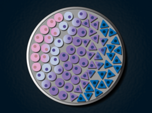
So, I joined a poop lab. I’ll let that one sink in. We work with stool samples so much that we have to make light of it. Stool jokes are commonplace, even encouraged, in lab meeting presentations. Everyone in the lab is required to make their own “poo-moji” after they join.

My poo-moji. What a likeness!

I did my inaugural microbial DNA extraction from stool samples last week. I was expecting worse; it didn’t smell nearly as bad as I expected. Still, running this protocol always has me thinking about the potential for things to end very badly:

  1. Place frozen stool in buffer
  2. Heat to 85 degrees C
  3. Vortex violently for 1 minute
  4. ….

Yes, we have tubes full of liquid poo, heated to nearly boiling temperature, shaking about violently on the bench! You can bet I made sure those caps were on tight.

Jokes aside, my interest in this field continues to grow the more I read about the microbiome. As a start, here are some of the genomics and methods topics I find interesting at the moment:

  • Metagenomic binning. Metagenomics often centers around working on organisms without a reference genome – maybe the organism has never been sequenced before, or it has diverged so much from a reference that it’s essentially useless. Without aligning to a reference sequence, how can we cluster contigs assembled from a metagenomic sequencing experiment such that a cluster likely represents a single organism?
  • Linked reads, which provide long-range information to a typical short read genome sequencing dataset. They can massively aid in assembly and recovery of complete genomes from a metagenome.
  • k-mer analysis. How can short sequences of DNA be used to quickly classify a sequencing read, or determine if a particular organism is in a metagenomic sample? This hearkens to some research I did in undergrad on tetranucleotide usage in bacteriophage genomes. Maybe this field isn’t too foreign after all!

On the biological side, there’s almost too much to list. It seems like the microbiome plays a role in every bodily process involving metabolism or the immune system. Yes, that’s basically everything. For a start:

  • Establishment of the microbiome. A newborn’s immune system has to tolerate microbes in the gut without mounting an immune overreaction, but also has to prevent pathogenic organisms from taking hold. The delicate interplay between these processes, and how the balance is maintained, is very interesting to me.
  • The microbiome’s role in cancer immunotherapy. Mice without a microbiome respond poorly to cancer immunotherapy, and the efficacy of treatment can reliably be altered with antibiotics. Although researchers have shown certain bacterial groups are associated with better or worse outcomes in patients, I’d really like to move this research beyond correlative analysis.
  • Fecal microbial transplants (FMT) for Clostridium difficile infection. FMT is one of the most effective ways to treat C. difficile, a infection typically acquired in hospitals and nursing homes that costs tens of thousands of lives per year. Transferring microbes from a healthy donor to a infected patient is one of the best treatments, but we’re not sure of the specifics of how it works. Which microbes are necessary and sufficient to displace C. diff? Attempts to engineer a curative community of bacteria by selecting individual strains have failed, can we do better by comparing simplified microbial communities from a stool donor?

Honestly, it feels great to be done with rotations and to have a decided lab “home.” With the first year of graduate school almost over, I can now spend my time in more focused research and avoid classes for the time being. More microbiome posts to come soon!

Deep learning to understand and predict single-cell chromatin structure

In my last post, I described how to simulate ensembles of structures representing the 3D conformation of chromatin inside the nucleus. Now, I’m going to describe some of my research to use deep learning methods, particularly an autoencoder/decoder, to do some interesting things with this data:

  • Cluster structures from individual cells. The autoencoder should be able to learn a reduced-dimensionality representation of the data that will allow better clustering.
  • Reduce noise in experimental data.
  • Predict missing points in experimental data.

Something I learned early on rotating in the Kundaje lab at Stanford is that deep learning methods might seem domain specific at first. However, if you can translate your data and question into a problem that has already been studied by other researchers, you can benefit from their work and expertise. For example, if I want to use deep learning methods on 3D chromatin structure data, that will be difficult because few methods have been developed to work on point coordinates in 3D. However, the field of image processing has a wealth of deep learning research. A 3D structure can easily be represented by a 2D distance or contact map – essentially a grayscale image. By translating a 3D structure problem into a 2D image problem, we can use many of the methods and techniques already developed for image processing.

Autoencoders and decoders

The primary model I’m going to use is a convolutional autoencoder. I’m not going into depth about the model here, see this post for an excellent review. Conceptually, an autoencoder learns a reduced representation of the input by passing it through (several) layers of convolutional filters. The reverse operation, decoding, attempts to reconstruct the original information from the reduced representation. The loss function is some difference between the input and reconstructed data, and training iteratively optimizes the weights of the model to minimize the loss.

In this simple example, and autoencoder and decoder can be thought of as squishing the input image down to a compressed encoding, then reconstructing it to the original size (decoding). The reconstruction will not be perfect, but the difference between the input and output will be minimized in training. (Source)

Data processing

In this post I’m going to be using exclusively simulated 3D structures. Each structure starts as 64 ordered 3D points, an 64×3 matrix with x,y,z coordinates. Calculating the pairwise distance between all points gives a 64×64 distance matrix. The matrix is normalized to be in [0-1]. The matrix is also symmetric and has a diagonal of zero by definition. I used ten thousand structures simulated with the molecular dynamics pipeline, with an attempt to pick independent draws from the MD simulation. The data was split 80/20 between training and

Model architecture

For the clustering autoencoder, the goal is to reduce dimensionality as much as possible while still retaining good input information. We will accept modest loss for a significant reduction in dimensionality. I used 4 convolutional layers with 2×2 max pooling between layers. The final encoding layer was a dense layer. The decoder is essentially the inverse, with upscaling layers instead of max pooling. I implemented this model in python using Keras with the Theano backend.

Dealing with distance map properties

The 2D distance maps I’m working with are symmetric and have a diagonal of zero. First, I tried to learn these properties through a custom regression loss function, minimizing the distance between a point i,j and its pair j,i for example. This proved to be too cumbersome, so I simply freed the model from learning these properties by using custom layers. Details of the implementation are below, because they took me a while to figure out! One custom layer sets the diagonal to zero at the end of the decoding step, the other averages the upper and lower triangle of the matrix to enforce symmetry.

Clustering single-cell chromatin structure data

No real clustering here…

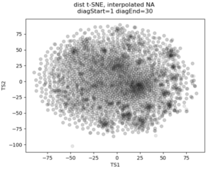
In the past I’ve attempted to visualize and cluster single-cell chromatin structure data. Pretty much any way I tried, on simulated and true experimental data, resulted the “cloud” – no real variation captured by the axes. In this t-SNE plot from simulated 3D structures collapsed to 2D maps, you can see some regions of higher density, but no true clusters emerging. The output layer of the autoencoder ideally contains much of the information in the original image, at a much reduced size. By clustering this output, we will hopefully capture more meaningful variation and better discrete grouping.


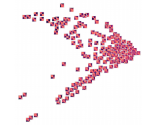
Groupings of similar folding in the 3D structure!

Here are the results of clustering the reduced dimensionality representations learned by the autoencoder. I’m using the PHATE method here, which seems especially applicable if chromatin is thought to have the ability to diffuse through a set of states. Each point is represented by the decoded output in this map. You can see images with similar structure, blocks that look like topologically associated domains, start to group together, indicating similarities in the input. There’s still much work to be done here, and I don’t think clear clusters would emerge even with perfect data – the space of 3D structures is just too continuous.

Denoising and inpainting

I am particularly surprised and impressed with the usage of deep learning for image superresolution and image inpainting. The results of some of the state of the art research are shocking – the network is able to increase the resolution of a blurred image almost to original quality, or find pixels that match a scene when the information is totally absent.

With these ideas in mind, I thought I could use a similar approach to reduce noise and “inpaint” missing data in simulated chromatin structures. These tasks also use an autoencoder/decoder architecture, but I don’t care about the size of the latent space representation so the model can be much larger. In experimental data obtained from high-powered fluorescence microscope, some points are outliers: they appear far away from the rest of the structure and indicate something went wrong with hybridization of fluorescence probes to chromatin or the spot fitting algorithm. Some points are entirely missed, when condensed to a 2D map these show up as entire rows and columns of missing data.
To train a model to solve these tasks, I artificially created noise or missing data in the simulated structures. Then the autoencoder/decoder was trained to predict the original, unperturbed distance matrix.

Here’s an example result. As you can see, the large scale features of the distance map are recovered, but the map remains noisy and undefined. Clearly the model is learning something, but it can’t perfectly predict the input distance map

Conclusions

By transferring a problem of 3D points to a problem of 2D distance matrices, I was able to use established deep learning techniques to work on single-cell chromatin structure data. Here I only showed simulated structures, because the experimental data is still unpublished! Using an autoencoder/decoder mode, we were able to better cluster distance maps into groups that represent shared structures in 3D. We were also able to achieve moderate denoising and inpainting with an autoencoder.

If I was going to continue this work further, there’s a few areas I would focus on:

  • Deep learning on 3D structures themselves. This has been used in protein structure prediction [ref]. You can also use a voxel representation, where each voxel can be occupied or unoccupied by a point. My friend Eli Draizen is working on a similar problem.
  • Can you train a model on simulated data, where you have effectively infinite sample size and can control properties like noise, and then apply it to real-world experimental data?
  • By working exclusively with 2D images we lose a lot of information about the input structure. For example the output distance maps don’t have to obey the triangle inequality. We could use a method like Multi-Dimensional Scaling to get a 3D structure from an outputted 2D distance map, then compute distances again, and use this in the loss function.

Overall, though this was an interesting project and a great way to learn about implementing a deep learning model in Keras!


Simulating 3D chromatin structure with molecular dynamics and loop extrusion

Much of the current evidence for the loop extrusion hypothesis comes from molecular dynamics simulations. In these simulations, DNA is modeled as a polymer, loop extruding factors with certain parameters are added into the mix, and the polymer is allowed to move around as if it were in a solvent. By running the simulation for a long time and saving conformations of the polymer at defined intervals, you can gather an ensemble of structures that represent how chromatin might be organized in a population of cells. Note that molecular dynamics is much different than MCMC approaches to simulating chromatin structure – here we’re actually simulating how a chromatin might behave due to physical and chemical properties.

In this post, I’m going to show you how you can run these molecular dynamics simulations for yourself. The simulations rely on the OpenMM molecular simulation package, the Mirnylab implementation of openmm-polymer and my own scripts and modification of the mirnylab code.

Ingredients

  • Install the required packages. See the links above for required code repositories. Note that it can be quite difficult to get openmm-polymer configured properly, so good luck…
  • Simulation is much quicker using a GPU
  • Pick your favorite chromatin region to simulate. In this example, we’re going to use a small region on chromosome 21.
  • Define CTCF sites, including orientation and strength. These will be used as blocking elements in the simulation. The standard is to take CTCF binding ChIP-Seq data for your cell type of interest, overlap the peaks with another track too add confidence and determine orientation (such as CTCF motifs in the genetic code or RAD21 binding data).
  • Define other parameters for the simulation, such as the time step and number of blocks to save. These can be found in the help text for the simulation script.

Check your parameters

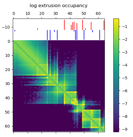
Before running a time consuming 3D polymer simulation, you can run simple test to see how the extruding factors are behaving in the simulation. This 2D map gives the probability of an extruder binding two sites along the linear genome, and is a good prediction for how the mean 3D structure will look. Briefly, there’s a logistic scaling function that transforms an arbitrary ChIP-Seq peak strength into a 0.0-1.0 interval. The scaled strength of the each site defines the probability that a LEF can slip past the site without stalling. Even though CTCF might form an impermiable boundary in reality, modeling this with a probability makes sense because we’re generating an ensemble of structures. You might need to tune the parameters of the function to get peak strengths to make sense for your ChIP-Seq data.

Loop extruder occupancy matrix. This gives the log transformed probability of a LEF binding two locations along the genome. CTCF sites for the example region of interest are shown above, with the color indicating directionality and height indicating strength. Notice how we already start to see domain-like structures!

Running the simulation

With all the above ingredients and parameters configured, it’s time to actually run the simulation. Here we will run for a short number of time steps, but you should actually let the simulation run for much longer to gather thousands of independent draws from the distribution of structures.

Using the code available at my github, run the loop_extrusion_simulation.py script. Here is an example using the data available in the repository

cd openmm-dna
python src/loop_extrusion_simulation.py -i data/example_ctcf_sites.txt -o ~/loop_extrusion_test --time_step 5000  --skip_start 100 --save_blocks 1000

Some explanation of the parameters: time_step defines how many steps of simulation are done between saving structures, skip_start makes the script skip outputting the first 100 structures to get away from the initial conformation, save_blocks means we will save 1000 structures total. There are many other arguments to the script, check the help text for more. In particular, the –cpu_simulation flag can be used if you don’t have a GPU.

If everything is configured correctly, you’ll see output with statistics on the properties of each block.

potential energy is 3.209405
bl=1 pos[1]=[10.9 14.2 5.8] dr=1.46 t=8.0ps kin=2.39 pot=2.24 Rg=9.084 SPS=235
Number of exceptions: 3899
adding force HarmonicBondForce 0
adding force AngleForce 1
Add exclusions for Nonbonded force
Using periodic boundary conditions!!!!
adding force Nonbonded 2
Positions...
loaded!
potential energy is 2.354693
bl=2 pos[1]=[11.4 14.1 6.0] dr=1.21 t=8.0ps kin=1.78 pot=2.09 Rg=9.278 SPS=333
...

Processing simulated structures

After simulation, I process the raw structures by trimming the ends (by the same amount of the –extend argument) and binning the points by taking the 3D centroid to reduce the resolution. As I’m trying to match experimental data with this simulation, I reduce the resolution to the same as the experimental data. Then I save the ensemble in a numpy array, which is much quicker to load for subsequent analysis. There’s a script to do this:

python src/process_simulated_structures.py -i ~/loop_extrusion_test -o ~/loop_extrusion_test/processed

Analysis of results

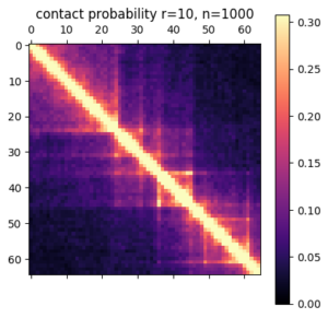
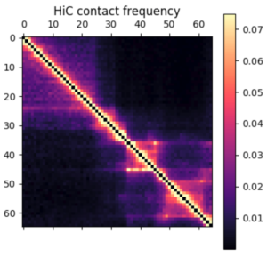
There are a few ways you can analyze the results after the simulation has finished. The obvious first step is to create an average contact map from the ensemble of structures. This plot is the most comparable to a Hi-C dataset.

Simulation contact probability at radius of 10. 1000 structures went into this plot.

Hi-C contact frequency for the same region in K562 cells. A great qualitative match, inluding domains and peaks!


Another common way to look at chromatin structure data is plotting contact probability as a function of genomic distance. This function is expected to decrease linearly on a log-log plot, with the slope giving evidence for mechanism for packing the underlying structures. You can look at the radius of the structures, how they cluster, and many other metrics. More on this to come later!

Is loop extrusion responsible for the 3D structure of the genome?

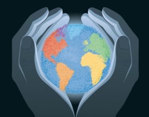
3D genome organization shapes genetics at all scales. Source: Nature 3D Genome Collection

It’s generally accepted biological knowledge that chromatin is organized in a complex and tightly-regulated manner inside the cellular nucleus. High-throughput chromatin conformation capture (Hi-C), microscopy experiments and computer simulations have added much to our knowledge of chromatin’s three dimensional organization. However, there still isn’t a consensus on the molecular mechanisms actually responsible for such organization!

A major advance in the past few years was the formalization of the loop extrusion hypothesis. Loop extrusion explains many features of experimental data – and I’m going to describe it in detail soon. However, we still don’t have conclusive mechanistic evidence that it is actually happening inside the nucleus. New research is continually adding to the body of evidence for the hypothesis, though, so it looks like loop extrusion is here to stay.

Loop extrusion, explained

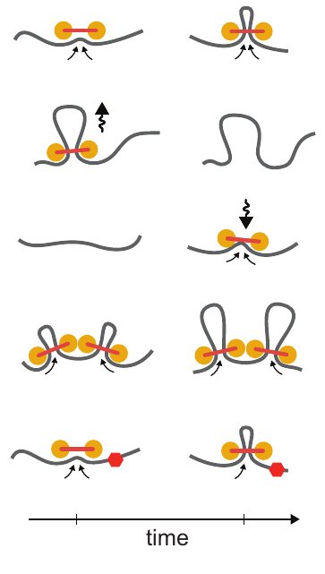
Loop extrusion dynamics. Extruders are shown as linked pairs of yellow circles, chromatin fiber shown in gray. From top to bottom: extrusion, dissociation, association, stalling upon encountering a neighboring extrusion comples, stalling at a blocking element (red hexagon). Taken from Figure 2 of [1]

Chromatin in the nucleus of the cell is organized in an incredibly robust and precise way. Over 2m of linear DNA has to fit into the nucleus, around 10µm in diameter. Each chromosome has to be faithfully replicated every time the cell divides, chromatin has to be “opened” and “closed” in response to external signals, and transcriptional machinery has to be able to access each gene to express mRNA and produce proteins. Past research has shown that the genome is organized at different levels (compartments, domains, sub-domains), and contains “peaks” of increased 3D interaction at specifically defined loci, often between binding sites for the transcription factor CTCF. Any mechanistic model for chromatin organization needs to take all of these factors into account.

Loop extrusion considers the action of extruding factors – most likely the proteins cohesin or condensin. Extruding factors are typically thought of as pairs of proteins with a fixed linker between them. They bind DNA and each member of the pair translocates along the polymer, effectively extruding a loop. Unhindered, an extrusion complex will process along the DNA until it dissociates. If an extrusion complex encounters another, both will stall at that position on the DNA. The model also considers blockers – most likely bound CTCF – that can stall extrusion complexes. Blockers are modeled to be directional (they only block extruders moving in one direction) and semi-permeable (they let an extruder pass with a certain probability). For a video explaining the action of loop extrusion, see this post.

Loop extrusion provides a simple unifying principle to explain 3D genome structure. Initially, the best evidence for this hypothesis came from simulation using molecular dynamics – simulating the action of loop extrusion complexes on a polymer constructed to mimic DNA. By placing blocking sites at locations where CTCF was bound in the genome, these simulations closely reconstructed experimental Hi-C data. In addition, loop extrusion can explain what Hi-C contact maps look like after removing CTCF binding sites with CRSIPR genome editing.

There’s a interesting history of the loop extrusion hypothesis – it’s actually not a completely novel idea for explaining genome architecture. A report in 1990 by Arthur Riggs [3] proposed “DNA reeling.” Then, Kim Nasmyth mentioned that an extrusion-like mechanism might play a role in separating sister chromatids  and genome organization in 2001 [4]. However, the idea was buried in a 75 page article. Nasmyth even discouraged the idea, “I give this example not so much because it is a serious candidate for the function of condensin (or cohesin for that matter) but rather because it illustrates the notion that condensin or molecules like it could have a very active role in folding and resolving chromatids.” As far as I can tell, loop extrusion went untouched until a publication by Alipour and Marko in 2012 [5], who proposed an extrusion-like mechanism could be used to compact mitotic chromosomes. Then, concurrent publications by the Mirny and Lieberman Aiden groups formalized the idea [1,2]. The timing of these publications was interesting – a preprint of one came out while the other was in review. However, the authors maintain that the ideas were developed independently.

Loop extrusion is a convincing hypothesis, but mechanistic explanation for it actually happening in the genome is lacking. A few recent publications have begun to address this, defining the proteins that are responsible and the parameters that govern their action. For example, Ganji et. al. [6] used single molecule imaging to visualize that condensin from S. cerevisiae could form loops on DNA, at a rate of up to 1500 bp/s. “Here, we provide unambiguous evidence for loop extrusion by directly visualizing the formation and processive extension of DNA loops by yeast condensin in real-time.”

Further biophysical experiments will likely give us more confidence about loop extrusion. In particular, evidence in human cells with human cohesin/condensin is lacking.

References

1. Fudenberg, G. et al. Formation of Chromosomal Domains by Loop Extrusion. Cell Reports 15, 2038–2049 (2016).
2. Sanborn, A. L. et al. Chromatin extrusion explains key features of loop and domain formation in wild-type and engineered genomes. PNAS 201518552 (2015).
3. Riggs, A. D. DNA methylation and late replication probably aid cell memory, and type I DNA reeling could aid chromosome folding and enhancer function. Phil. Trans. R. Soc. Lond. B 326, 285–297 (1990).
4. Nasmyth, K. Disseminating the Genome: Joining, Resolving, and Separating Sister Chromatids During Mitosis and Meiosis. Annual Review of Genetics 35, 673–745 (2001).
5. Alipour, E. & Marko, J. F. Self-organization of domain structures by DNA-loop-extruding enzymes. Nucleic Acids Res 40, 11202–11212 (2012).
6. Ganji, M. et al. Real-time imaging of DNA loop extrusion by condensin. Science eaar7831 (2018). doi:10.1126/science.aar7831

Down and up the California coast

With 11 days left to go before move-in at Stanford, I had only just made it to California. There was still so much to see! I headed down to the Bay to see some friends in Oakland (and for a much needed shower!) and then out to the coast. Route 1 was still closed south of Big Sur, so I stopped for two nights in Pfeiffer Big Sur State Park to explore the surrounding trails and beaches.

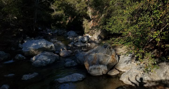
Climbing boulders in the Big Sur River. See the shadow at the bottom?

Another great stop was in Santa Cruz, home of the well-known Santa Cruz bike company. They let you take out a top of the line demo bike for $20, which is a steal for a whole day of riding. I rented a Tallboy 29er and was blown away with how it felt compared to my Specialized hardtail I had been riding all summer. Dual suspension, hydraulic disk breaks, 1x gearing, tubeless tires and a riser seat post made the climbs a breeze and rocky descents feel like smooth pavement. I was sold. Now to scare up another $3k for a new bike…

Great views with the Santa Cruz.

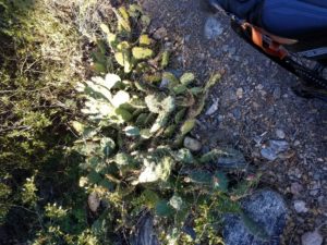
I stayed with some friends in Newport Beach and spent the weekend surfing and soaking up the SoCal sun. Afterwards, it was back into the wilderness for a short two-day bikepacking trip in Big Bear, CA. The environment here was much closer to a desert, and I learned that tires seem to magically attract cactus needles. I was limping along on patched tubes by the time I got back to the car.

In the morning, I was cooking breakfast by a river and minding my own business. Off in the distance I heard some rustling in the bushes and tensed up. Silence for a minute, and then I spotted a bear investigating the smells from my camp! Luckily he scared off when I started clapping and shouting. Having asserted my dominance over this section of the river, I thought I was safe to continue my breakfast. But no! A second, different bear also decided it was time to say hi! This one got much closer before I heard it, and have me quite a scare when it popped its head over the riverbank. I promptly packed up and left the bears to their spot after the second encounter.

Departing for a night out in Big Bear. I was much better at packing this time around!

Cacti and flats became a theme of this trip.


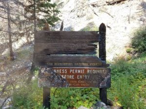
This sign had seen better days…

Driving West and a Week in Tahoe

After the eclipse, a few friends joined me for the drive West into California. Already four thousand miles of solo driving in, I was grateful for the company! We stopped at the great salt flats in Utah along the way, before camping just north of Lake Tahoe for the night.

Salt flats for as far as the eye can see.

Morning yoga on the foggy lake.


Everyone else had a flight to catch or school to start in the Bay, so I stayed behind in Tahoe for about a week. This was my first time in Tahoe in the summer, and I LOVED it. Tahoe is basically a playground for adults. Any sport you want to do, there’s the place for it within a 30 minute drive. My days were filled with mountain biking to crystal clear alpine lakes, kayaking lake Tahoe and picnicking on islands and going to a reggae festival in South Lake Tahoe.

It takes a few hours to bike to Dardanelles lake, but you’re rewarded with crystal clear water and almost complete solitude.

Sierra meadows with the sun low in the sky.


Kayaking on the lake. There are so many inlets, waterfalls and rock diving spots to explore!

The “Tea House” on Fannette Island in Emerald Bay.


I was amazed by the Tahoe beaches, I felt like I was in the tropics.

This rock was being swallowed alive!

Jasper, Glacier, Eclipse

After finishing the bikepacking trip and a well-deserved recovery meal, was headed back up North for a few days in Jasper National Park. Situated a few hours North of Banff, Jasper is a more quite and remote park in the Canadian Rockies. The drive takes you through Mountains and Glaciers, with many places to pull over for views and a short hike along the way. A highlight is Athabasca Glacier, where you can walk right up to an real live glacier!

Breakfast IS the most important meal of the day!

Athabasca Glacier, slowly receding into the distance


I spent a few days of exploring the hiking and mountain biking trails in Jasper, and one excellent night soaking at Miette Hot Springs. Overall I preferred Jasper to Banff – it doesn’t have the rich resort feel in town, is less crowded, and nature feels closer by.

Back into the United States and a quick stop in Glacier National Park for a day hike and overnight camp.

Wildflowers below a Glacier in Glacier NP.

The next destination was Lander, Wyoming, directly in the path of the total solar eclipse on August 21. Luckily, a friend grew up in Wyoming and her house was directly in the path of totality! Her parents were kind enough to let a few friends and I spend some time on their ranch to see this once in a lifetime event. On the day, we camped out ahead of time with snacks and drinks and waited for the moon to eclipse the sun….

Sunglasses AND eclipse glasses. Take that solar rays!

A few seconds of night during totality


I didn’t take any photographs of the sun during the event, but if you didn’t get a chance to see the eclipse in person you can find way better photos online. I can say that totality was unlike any natural event I’ve experienced – the rapidly darkening sky, chilling air, and hushing environment around you. Look up and see the rainbow effects around the moon and complete eclipse of the sun. 30 seconds I’m not going to forget any time soon.

Bikepacking in Banff

The main attraction for this part of the trip was a 3-day bikepacking trip from Banff, south into British Colombia, and back again. This was my first time bikepacking so I had a lot to learn, even before starting the trip. That learning began with planning a route — Nowhere in Banff National Park can you park your car at a trailhead and head out into the wilderness. You need a permit (for everything in Canada, it seemed) and a prescribed route to avoid coming back to a towed car. Very different than the East Coast where I grew up hiking and backpacking. I ended up starting the trip from Canmore, South of Banff and out of the national park for this reason.

The second learning experience came with packing up my gear. I knew size more than anything was going to be a priority on this trip, so I had optimized my packing to take that into account. I had two Ortlieb bikepacking bags on the handlebars and saddle, a small tool bag on the frame, and a backpack for water, extra layers, and accessible snacks. Here’s a shot of everything I brought on the trip for 3 days. I was expecting rain and highly variable temps so lots of layers were key!

Organizing supplies for a 3-day trip. This all had to fit in the two bike bags or on my back, so weight and size was a priority.

Packed up and ready to hit the trail.


In the end I wore every layer I brought at some point, used most of the tools in my kit and ate every last bit of food, so my packing might have been a bit on the light side. Fitting all this into bags was also a challenge, and I had to pull over to adjust the load many times in the first day of the trip.

My planned route was the High Rockies Trail, a singletrack trail that runs south from Canmore. I originally wanted to bike the Great Divide trail, which is famous for spanning the continental divide from Canada to Mexico. However the Great Divide runs on gravel roads for much of Canada. The High Rockies parallels the Great Divide and gives you a much more exciting ride. I had a simple map of the trail from Banff, but I ended up doing most of the navigation on my phone with the Trailforks app (indispensable on this road trip).

Here are some highlights from the three days out in the wilderness:

Sunrise looking out over the mountains.

Flowers start to grow back after a wildfire.

Setting up a kitchen on a bridge. Oats and coffee for breakfast.

This bridge was under construction. It would have saved me a few miles and a thousand feet of elevation, so I thought about trying my balance…

Panoramic views everywhere you pulled over.

At the end of three days I was exhausted, hungry and thrilled to make it back to my car. I made a few mistakes on this first bikepacking trip and learned many lessons. I still had a great time in the wilderness, but next time would pack better shoes, more food, set less optimistic distance goals when riding singletrack and pack my load better from the get-go.

Getting to know Banff

I was thrilled to finally arrive in Banff. After long days in the car, and hours of cruise-controlled monotony across the plains of Canada, the chilled mountain air was a welcome feeling. I immediately took the bike out for a ride along some trails by a river, and up into the mountains along a path with more tree roots than I’ve ever seen before.

There were active wildfires in BC and Alberta, resulting in a hazy sky for most of the trip.

The suspension took a beating on this one.


After the climb I was rewarded with excellent views of the mountains and the town of Banff nestled below.


The next day I explored the Lake Louise area. The striking blue color of Lake Louise is something you have to see in person to believe – a photo doesn’t do it justice. Get there early in the morning, before the tourists and canoes fill the frame, and you’ll have a sight to remember.

The blue of the lake and the morning haze were a mesmerizing combination. I learned that the blue comes from glacial flour – small particles of silt that are ground up by glaciers and washed into the lake.

Hiking upward from Lake Louise, you come upon a few alpine lakes and waterfalls to cool you off. It was August, but you can still see traces of snow up in the bowl! The top of the trail also has a teahouse where you can relax from the hike with a hot drink.

Plenty of other tourists to take your photo, even early in the morning.

Catching Lake Louise through the trees as I hiked upward.

Lake Agnes – a few miles up the trail from Louise.


Moving to California, the long way

I’m starting a PhD in Genetics at Stanford in the fall. The plans are set, I’ve moved out of my apartment, and  thrown away A LOT of clutter from the past year. All that’s left is to physically get myself to California. Can you think of a better way than taking a month to drive across the country with a mountain bike in the car?

I was READY to hit the road. This would be the second time around the country for the Saab!

The first main destination was Banff National Park in Alberta, Canada. The Canadian Rockies have amazing sights, wildlife and trails for hiking and biking – I encourage anyone who hasn’t been to take a trip.

Some highlights of the first few days, in pictures:

An Amish produce stand I found by following some hand painted signs off the highway.

Homemade summer sausage that weighed over a POUND AND A HALF. This was a part of every dinner for the next two weeks or so.

It’s not camping without a few elaborate dinners cooked over a camp stove.

Sunset over Lake Superior. Can you see the freight train in the distance, with the light on the front?

I learned that Ontario is filled with small lakes. It seems like every time I pulled over to take a break or have lunch, I had a chance to get in the water for a quick swim.

Warning: I took a lot of selfies on this trip, had to do something to keep myself company!

A truck on the side of the road, on fire, at 7am. What?!


It was a long 3 days of driving to get from Massachusetts to Calgary. Especially the last 24 hours or so through the plains of Manitoba and Saskatchewan. But long hours on the highway paid off, because I got to Calgary fairly quickly. Eventually, the mountains were within reach!

The Canadian Rockies loom in the distance. I knew I was getting close.

45+ hours of driving, 2700 miles later…